Excel spreadsheets can quickly become large and complex, with data flowing between sheets and many people accessing the file. To protect certain rows from being edited accidentally, Excel allows you to lock cells or entire rows. Locking rows is a simple but useful feature that can help prevent errors and preserve data integrity in your spreadsheets.
In this blog post, we’ll explain what it means to lock rows in Excel and walk you through the easy steps to lock rows on your own worksheets. Whether you’re looking to lock individual rows or lock all rows on your spreadsheet, locking rows is a great way to safeguard your data when sharing Excel files between multiple users. Read on to learn how to use this excellent Excel feature to lock down rows in your spreadsheets!
Why Locking Rows in Excel Matters
Before we dive into the nitty-gritty of the process, let’s understand why locking rows in Excel is such a vital skill. Imagine you have a large dataset with hundreds of rows and columns. You’ve put a lot of effort into formatting, organizing, and adding formulas to your worksheet.
The last thing you want is to accidentally overwrite or misplace important data. This is where locking rows comes to the rescue.
Protecting Your Data
Locking rows in Excel is a crucial step to protect your data from inadvertent modifications. It ensures that specific rows remain visible and stationary, no matter how much you scroll through your spreadsheet. This is particularly important when working with headers, summaries, or important reference data.
Enhancing Readability
When you lock rows, you also enhance the readability of your worksheet. As you navigate through a large dataset, having essential information at the top of your screen, no matter how far down you’ve scrolled, is invaluable. It keeps your data context intact and saves you from constant scrolling up and down.
How to Lock Rows in Excel: A Step-by-Step Guide
Now, let’s get to the heart of the matter. We will walk you through the process of locking rows in Excel, step by step. Follow these instructions carefully to ensure a smooth and productive experience.
Step 1: Open Your Excel Workbook:
Begin by opening your Excel workbook and navigating to the worksheet where you want to lock rows. Make sure you’re working on the specific sheet where this feature is needed.
Step 2: Select the Rows to Be Locked:
Click and drag your cursor over the rows you wish to lock. These rows should be at the top of your spreadsheet and contain critical data or headers. Your cursor should be on the row that is below the ones that you want to freeze.
Step 3: Access the Freeze Panes Option:
Go to the “View” tab on the Excel ribbon. Within the “Window” group, you will find the “Freeze Panes” option. Click on it to reveal a drop-down menu.
Step 4: Choose Your Freezing Option:
In the drop-down menu, you have three options:
- “Freeze Panes”: This option will freeze the selected rows, making them constantly visible as you scroll.
- “Freeze Top Row”: This choice locks only the top row.
- “Freeze First Column”: This option locks the first column.
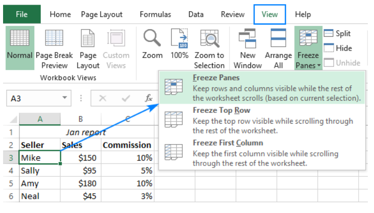
Select the option that best suits your needs. In our case, we are focusing on locking rows, so choose “Freeze Panes.”
Step 5: Verify Your Rows Are Locked:
After selecting “Freeze Panes,” you will notice a faint line appear below the locked rows. This line indicates that the chosen rows are now frozen in place.
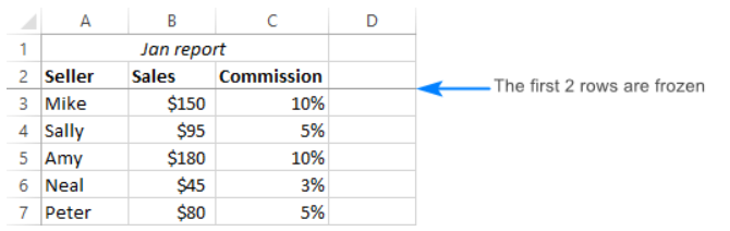
Step 6: Test It Out:
To ensure everything is working as intended, try scrolling down your worksheet. You will notice that the locked rows remain in place, providing continuous access to essential data.
Tips for Effective Row Locking
To make the most of this Excel feature, here are some additional tips:
- Unfreezing Rows: If you ever need to unfreeze the rows, return to the “Freeze Panes” option and choose “Unfreeze Panes.”
- Combining with Filters: Locking rows can work in conjunction with filters. You can easily filter your data while keeping your critical rows in view.
- Save Your Workbook: Remember to save your workbook regularly, especially after locking rows. This ensures that your preferences are retained.
- Customizing Freeze Panes: You can lock multiple rows by selecting a cell in the row just below the last row you want to freeze. Then, choose “Freeze Panes.”
Conclusion
Mastering the skill of locking rows in Excel is a game-changer for anyone working with large datasets. It safeguards your data, enhances visibility, and streamlines your workflow. Whether you’re a financial analyst, project manager, or a small business owner, this knowledge will elevate your Excel proficiency.
Unlock the power of Excel by learning how to lock rows, and watch your productivity soar to new heights. It’s a simple yet invaluable tool that can make a world of difference in your daily tasks and projects.