Whether you’re a business professional, a student, or someone who simply wants to make sense of data, Excel’s average function is a powerful tool that can simplify complex calculations and help you draw meaningful insights from your data sets.
In this comprehensive guide, we’ll walk you through everything you need to know about calculating averages in Excel, from the basics to advanced techniques. By the end of this article, you’ll have a deep understanding of how to use Excel to calculate averages effectively and efficiently.
Understanding the Average Function in Excel
Excel, as part of Microsoft Office’s suite of productivity tools, is widely used for data analysis and manipulation. One of its most commonly used functions is the AVERAGE function. The AVERAGE function allows you to calculate the average, or mean, of a set of numbers. It is an invaluable tool for a wide range of applications, including:
Data Analysis
Data analysts often use Excel to process and analyze large datasets. The AVERAGE function helps in summarizing data and making it more understandable. It can be applied to various scenarios, such as sales figures, survey results, or test scores.
Financial Analysis
In the financial world, Excel is a go-to tool for calculating financial metrics. The AVERAGE function can be used to calculate the average return on investment (ROI), average monthly expenses, or any other financial performance indicator.
Academic Research
Students and researchers use Excel for a multitude of tasks. When dealing with research data, the AVERAGE function helps in calculating the mean value of variables, making it easier to draw conclusions and identify trends.
Calculating Average in Excel
Using Excel’s Ribbon for Averages
When it comes to finding the average of a set of numbers in Excel, the ribbon is your best friend. Here’s a step-by-step guide to using this user-friendly feature:
- Open Your Spreadsheet: Start by opening your spreadsheet containing the numbers you wish to average.
- Select Your Numbers: In your spreadsheet, select the range of numbers for which you want to find the average.
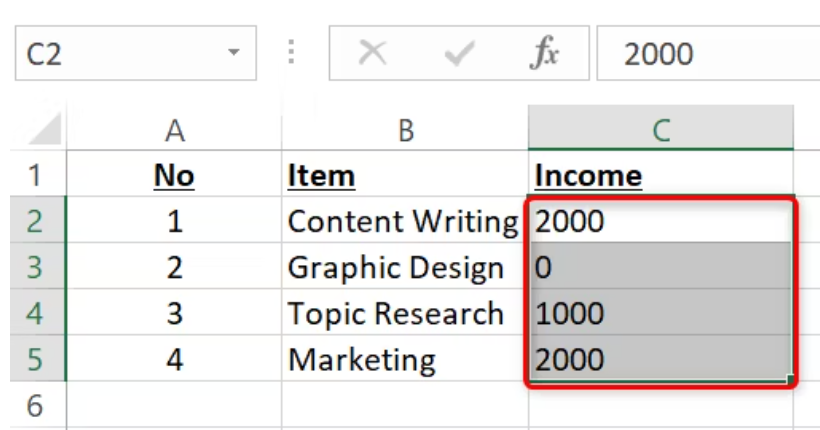
- Navigate to the “Home” Tab: Look for the “Home” tab in Excel’s ribbon, usually located at the top.
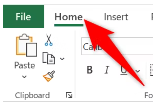
- Access the “Average” Option: Within the “Home” tab, you’ll find the “Editing” section. Click on the down-arrow icon next to the “Sum” option to reveal a dropdown menu.

- Choose “Average”: From the expanded menu, select the “Average” option.

- Excel will then swiftly calculate and display the average at the end of your selected cells.

It’s that simple! Using the ribbon option can save you time and effort when you need a quick average calculation.
Calculating Averages with Excel’s AVERAGE Function
If your numbers are not in a continuous row or column or if you prefer entering values directly into a formula, Excel’s AVERAGE function is your go-to tool. Follow these steps:
- Open Your Spreadsheet: Begin by opening your Excel spreadsheet.
- Select the Destination Cell: Click on the cell where you want to display the average.

- Enter the AVERAGE Function: In the selected cell, type the following function and press Enter, replacing “C2” and “C5” with the range that holds your numbers:
=AVERAGE(C2:C5)

- For Non-Contiguous Cells: If your numbers are spread across non-contiguous cells, you can specify each cell individually within the AVERAGE function. Separate the cells with commas, like so:
=AVERAGE(D2, E2, F2)
- Directly Enter Numbers: To input numbers directly into the formula, use commas to separate them, like this:
=AVERAGE(10, 15, 20)

- View the Result: Once you’ve entered the formula, press Enter, and Excel will display the average in your selected cell.

This method provides more flexibility, especially when dealing with scattered data.
Calculating Averages in Excel, Excluding Zeros
Sometimes, you might want to calculate an average while ignoring zeros in your dataset. Excel can do this efficiently with the AVERAGEIF function. Here’s how:
- Open Your Spreadsheet: Start by opening your Excel spreadsheet.
- Select the Destination Cell: Choose the cell where you want to see the result.
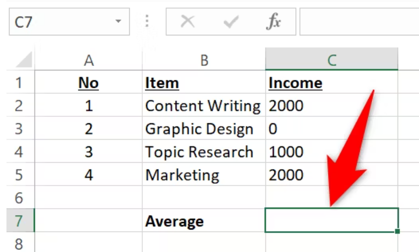
- Use the AVERAGEIF Function: In the selected cell, type the following function, replacing “C2” and “C5” with your number range:
=AVERAGEIF(C2:C5, “>0”)
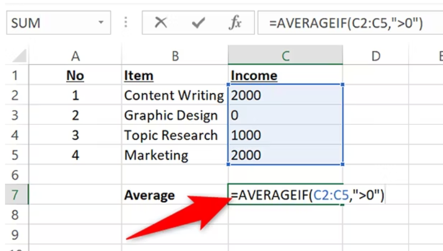
- Result Without Zeros: Once you’ve entered the formula and pressed Enter, Excel will calculate the average while ignoring any cells that contain zeros.
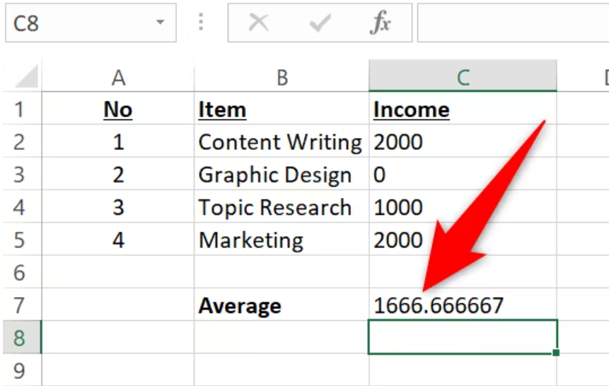
And there you have it! Excel’s AVERAGEIF function makes it easy to obtain the average you need while excluding undesired zeros from your calculation.
Conclusion
In conclusion, mastering Excel’s average calculations can significantly enhance your data analysis capabilities. Whether you prefer using the ribbon for quick averages or leveraging Excel’s AVERAGE function for more specific needs, these methods will undoubtedly make your spreadsheet tasks more efficient and accurate. Happy calculating!
