Excel, a powerhouse in data manipulation, becomes even more formidable when you unlock the potential of advanced lookup functions like INDEX and MATCH. In this comprehensive guide, we delve into the intricacies of these functions, offering practical insights and examples to elevate your Excel proficiency to new heights. By the end, you’ll not only understand their applications but also be equipped to use them seamlessly, enhancing your Excel capabilities.
Understanding the Power of MATCH
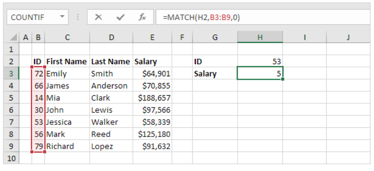
At the core of advanced Excel lookups lies the MATCH function. Its purpose is simple yet profound – determining the position of a value within a specified range. Consider this example:
=MATCH(53, B3:B9, 0)
In this instance, the function tells us that the value 53 is located at position 5 in the range B3:B9. The third argument (0) ensures an exact match, a crucial detail for precision in your data analysis.
Unveiling the Dynamics of the INDEX Function
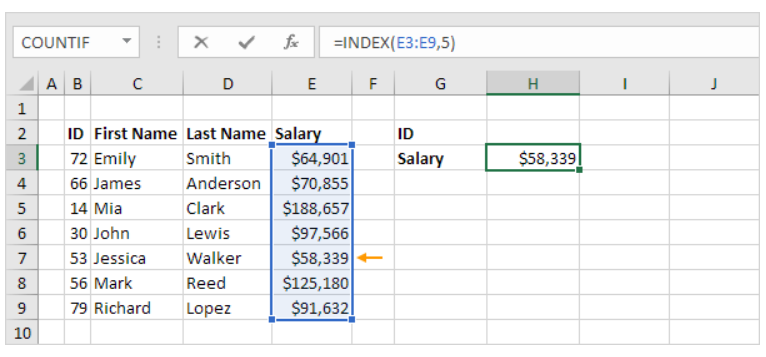
Complementing the MATCH function is the formidable INDEX. Unlike MATCH, INDEX fetches a specific value within a one-dimensional range. Observe the following formula:
=INDEX(E3:E9, 5)
Here, INDEX retrieves the fifth value in the range E3:E9. As we delve deeper, we’ll explore how combining MATCH and INDEX elevates your ability to perform intricate data retrievals.
Combining Index and Match: A Step-by-Step Guide
The true prowess of these functions comes to light when they work together. Replace the static value in the INDEX function with the dynamic output of MATCH, creating a dynamic synergy:
=INDEX(E3:E9, MATCH(53, B3:B9, 0))

This dynamic fusion enables you to efficiently look up information, as showcased in our example of retrieving the salary corresponding to ID 53.
Navigating Two-way Lookups with Finesse
As your Excel proficiency grows, so do the challenges. The INDEX function proves invaluable for two-dimensional lookups. The syntax evolves slightly:
=INDEX(range, MATCH(row_value, row_range, 0), MATCH(column_value, column_range, 0))

With this, you can seamlessly navigate the vast sea of data in Excel, extracting precisely what you need, whether it’s names, figures, or any other crucial information.
Achieving Case-sensitive Lookup Precision
While the default setting of the VLOOKUP function is case-insensitive, you may encounter scenarios where case-sensitivity matters. Enter INDEX, MATCH, and EXACT:
=INDEX(salary_range, MATCH(TRUE, EXACT(lookup_value, name_range), 0))

This nuanced formula ensures the correct match, making a distinction between MIA Reed and Mia Clark, a level of precision often indispensable in professional data analysis.
Overcoming Limitations with Left Lookup
The traditional VLOOKUP function restricts you to rightward searches. However, the dynamic duo of INDEX and MATCH allows for a left lookup. By reversing the order of your data, you can employ this formula:
=INDEX($E$4:$E$7, MATCH(A2, $G$4:$G$7, 0))

This opens up new possibilities, giving Excel the capability to look to the left for enhanced data retrieval.
Mastering Two-column Lookups for Precision
In scenarios where a single criterion falls short, elevate your game with a two-column lookup using INDEX and MATCH. The formula below illustrates how to fetch data based on multiple criteria:
=INDEX(salary_range, MATCH(1, (name_range= “James Clark”) * (position_range = “Manager”), 0))

This advanced technique ensures accuracy, fetching James Clark’s salary without confusion with James Smith or James Anderson.
Proximity Matters: Achieving the Closest Match
Navigate the nuances of data columns by utilizing INDEX, MATCH, ABS, and MIN to find the closest match to a target value:
=INDEX(data_column, MATCH(MIN(ABS(data_column – target_value)), ABS(data_column – target_value), 0))

Precision in Excel is not a luxury but a necessity, and this formula ensures you find the closest match with finesse.
Excel 365 and Excel 2021 Upgrade: Enter XLOOKUP
For those fortunate enough to have Excel 365 or Excel 2021, embrace the streamlined efficiency of XLOOKUP. Replacing the need for INDEX and MATCH, XLOOKUP simplifies the process with enhanced features.
=XLOOKUP(H2,B3:B9,E3:E9)

Upgrade your Excel experience with this powerful function, offering simplicity and additional advantages over traditional INDEX and MATCH methods.
In Conclusion
In Excel mastery, combining the INDEX and MATCH functions reigns supreme. From basic lookups to intricate two-column searches, these functions empower you to navigate and extract data with precision. Whether you stick to the classics or embrace the efficiency of XLOOKUP, your Excel journey has just ascended to new heights.