The INDEX MATCH combination is one of the most powerful lookup formulas in Excel. It allows you to pull data from a table based on a row and column match.
In this comprehensive guide, you will master the INDEX MATCH function in Excel through easy step-by-step examples. So let’s get started learning how to use INDEX MATCH in Excel!
What is the INDEX MATCH Formula in Excel?
The INDEX MATCH formula is a combination of two Excel functions:
- INDEX – Returns value in a cell based on row and column number
- MATCH – Finds the position of the lookup value in row/column
Combined together, INDEX MATCH allows you to look up values by matching on both vertical and horizontal criteria.
For example, you can find someone’s height by matching their name (vertically) and the column with ‘Height’ header (horizontally). This makes INDEX MATCH more powerful and flexible than VLOOKUP alone.
Now let’s see how each function works before putting them together.
How the INDEX Function Works in Excel
The INDEX function returns the value of a cell based on the row and column number specified.
The syntax is:
=INDEX(table_array, row_num, column_num)
Where:
- table_array – Full data table you want to reference
- row_num – Row number in the table
- column_num – Column number in the table
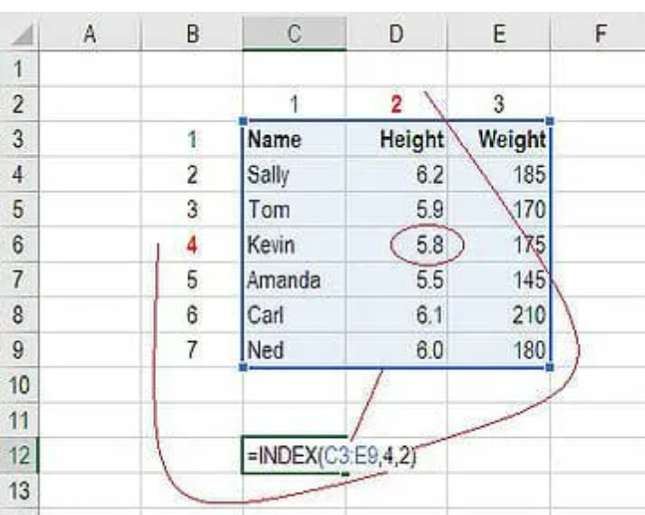
For example, in this table to find Adam’s height:
=INDEX(C3:E9,4,2)
This returns 5’8″ by matching 4th row and 2nd column.
INDEX is useful for lookups when you know the exact row and column to match. For dynamic lookups, it needs to be combined with MATCH.
How the MATCH Function Works in Excel
The MATCH function finds the relative position of a lookup value in a range.
The syntax is:
=MATCH(lookup_value, lookup_array, match_type)
Where:
- lookup_value – Value to find a match for
- lookup_array – Range to search in
- match_type – 1 for exact match or 0 for approximate
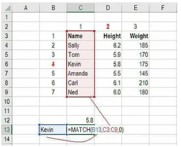
For example, to find Kevin’s row number in the table:
=MATCH(B13,C3:C9,0)
This returns 4 as Kevin is in 4th row.
To find the Height column number:
=match(B14,C3:E3,0)

This returns 2 as Kevn’s height is in the 2nd column.
MATCH gives the relative position, which can then be fed into INDEX.
How to Combine INDEX and MATCH in Excel
The full INDEX MATCH formula combines the row and column numbers from MATCH into the INDEX function.
The syntax is:
=INDEX(table_array, MATCH(row_lookup, row_range, 0), MATCH(column_lookup, column_range, 0))
Breaking this down:
- table_array – Full data table
- row_lookup – Value to match for row
- row_range – Range to search for row_lookup
- column_lookup – Value to match for column
- column_range – Range to search for column_lookup
Putting this together in our example:
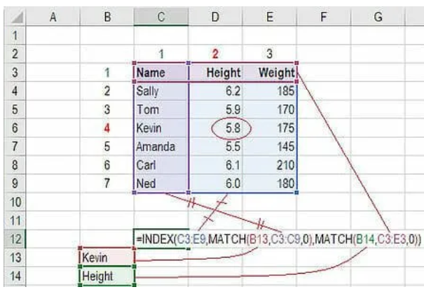
To look at Kevin’s Height:
- MATCH Kevin’s name to get row number:
=MATCH(B13,C3:C9,0) // Returns 4
- MATCH Height to get column number:
=match(B14,C3:E3,0) // Returns 2
INDEX with row_num and column_num:
=INDEX(C3:E9,4,2)) // Returns 5’8″
The combined formula is:
=INDEX(C3:E9,MATCH(B13,C3:C9,0),match(B14,C3:E3,0))
This dynamic formula works no matter where Kevin is in the table.
Using INDEX MATCH for Dynamic Lookups in Excel
The real power of INDEX MATCH comes from its dynamic lookups. Let’s see a few examples:
- Lookup someone’s weight by name and Weight header
- Get exam scores by student and subject
- Find email by manager and Email column header
The INDEX MATCH formula stays the same – only the lookup values need to change. No matter where columns move or data changes, the formula will continue returning the right lookup values. This makes INDEX MATCH ideal for dynamic reports and dashboards.
Use INDEX MATCH to Perform Data Analysis in Excel
You can use INDEX MATCH to perform many data analysis tasks in Excel:
- Lookup values from another sheet/workbook
- Return value from previous row/column
- Lookup with conditions (age >30)
- Vertical and horizontal approximate match
- Lookup based on multiple criteria
- Use in calculated columns to create reports
The beauty is that a single INDEX MATCH formula can handle all these scenarios by just changing the lookup values and ranges.
Some examples:
- Lookup manager for rep based on region
- Get forecast amount based on state and month
- Find the price for a product variant
- Get the latest Polls for today’s date
The possibilities are endless!
Variations with 0, 1, -1 Match Types in MATCH
The match_type argument in MATCH allows for powerful lookup variations:
- 0 finds the exact match
- 1 finds the closest match greater than the lookup value
- -1 finds the closest match lesser than the lookup value
Using 1 and -1 allows you to look up ranges and interpolate values.
For example:
- Lookup commissions for sales amount between brackets
- Get tax rate for income between tax slabs
- Lookup discount percentage for order quantity range
This adds a whole new dimension to your lookups!
Troubleshooting Errors in INDEX MATCH Formula
Some common errors and how to fix them:
- #N/A – Check for typos in lookup value
- #REF! – Check for wrong range reference
- #VALUE – Use correct match_type (0/1/-1)
- Wrong lookup – Double check row/column lookups
- Columns mismatched – Match column_num and column_lookup ranges
Should You Use INDEX MATCH or VLOOKUP?
While VLOOKUP is simpler, INDEX MATCH is more powerful and flexible.
When to use VLOOKUP:
- Simple vertical lookup from the table on the left
- The exact match on the first column
- Fixed references to the lookup table
When to use INDEX MATCH:
- Lookup values across columns and rows
- Dynamic lookups from any data layout
- Lookup values across sheets or workbooks
- Vertical and horizontal approximate match
- More complex data analysis
As you can see, INDEX MATCH can handle a lot more lookup scenarios. So take the time to learn it – it will supercharge your Excel skills!
Conclusion
Mastering the INDEX MATCH combination unlocks sophisticated lookup and data analysis skills in Excel. In this comprehensive guide, you gained the knowledge to leverage the power of INDEX MATCH for your own reports and dashboards.
We covered how INDEX and MATCH work individually, combining them for advanced lookups, dynamic matching on rows and columns, variations with match types, troubleshooting errors, and when to use this combo over VLOOKUP.
With concerted practice, you can now become adept at using INDEX MATCH to streamline complex lookups, powerful analysis, and efficient data processing in Excel. The time invested in learning this versatile technique will pay long-term dividends in boosting your spreadsheet productivity.