Are you looking to enhance your Excel skills and unlock the power of data manipulation? Look no further than the HLOOKUP formula in Excel. This versatile function allows you to search and retrieve values from horizontal sequences, providing you with the ability to organize and analyze data effortlessly.
In this comprehensive guide, we will explore the syntax, usage, and various examples of the HLOOKUP formula to empower you with the skills to become an Excel data ninja.
Syntax of HLOOKUP Formula in Excel
Before diving into the practical applications, let’s familiarize ourselves with the syntax of the HLOOKUP formula. Understanding each component of the formula will enable you to leverage its full potential effectively.
HLOOKUP Formula
=HLOOKUP(Lookup value, table, row_index, [True or False])
Now, let’s break down the syntax and explore each element:
Lookup value: This represents the value you want to search for within the data table.
Table: Refers to the range or data table where you want to find the value.
Row_index: Specifies the row number that contains the desired value.
True or False: This parameter determines the type of match you want to perform. Use 0 or False for an exact match and 1 or True for an approximate match.
It is crucial to choose the appropriate match type depending on the nature of your data. Exact matches are suitable for scenarios like finding sales figures or temperatures, while approximate matches are useful when dealing with ranges such as percentages.
How to Use the HLOOKUP Formula in Excel
Now that we have grasped the syntax of the HLOOKUP formula, let’s explore its practical application through a series of examples.
Example 1: Finding Monthly Sales
Suppose you have a sales data table containing six months of data, and you want to retrieve the sales figure for a specific month. Let’s use the HLOOKUP formula to find the sales for April.

HLOOKUP Formula for the above example
=HLOOKUP(B4, B1:G2, 2, 0)
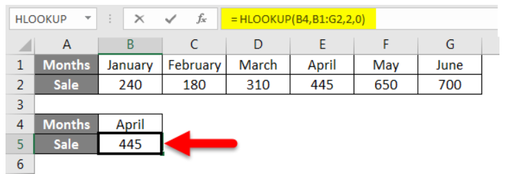
After typing in the HLOOKUP formula, press the Enter button
In this example:
- The lookup value (B4) represents April, the month we want to retrieve sales data for.
- B1:G2 is the range or table where the formula will search for the value.
- The row index (2) indicates the row containing the desired result.
- By setting the match type to 0, we ensure an exact match.
Example 2: Subject-wise Marks
Suppose you have a data table that displays subject-wise marks for different students. Let’s find out the marks in English for a specific student named Cole.

HLOOKUP Formula for the above example
=HLOOKUP(E1, B1:G4, 3, 0)

Once you’ve put in the formula, hit the enter button to get the final results

In this example:
- The lookup value (E1) represents Cole’s name.
- B1:G4 is the range or table where the formula will search for the value.
- The row index (3) indicates the row containing the desired result.
- Once again, we set the match type to 0 for an exact match.
Example 3: Multi-Criteria Lookup
Let’s say we want to find the marks in Maths for students who scored 75 marks in Science in the above example. We can use the HLOOKUP formula to accomplish this task.
HLOOKUP Formula for Example 3
=HLOOKUP(75, B2:G4, 3, 0)

Once again, hit enter to get the desired results

In this example:
- The lookup value (75) represents the score in Science.
- B2:G4 is the range or table where the formula will search for the value.
- The row index (3) indicates the row containing the desired result.
- By setting the match type to 0, we ensure an exact match.
Example 4: Employee Sales
Suppose you have a data table representing sales made by employees, and you want to find the sales figure for a specific employee using their ID.

HLOOKUP Formula for this case
=HLOOKUP(B8, B1:F6, 5, 0)

Now press the Enter Key to get your results
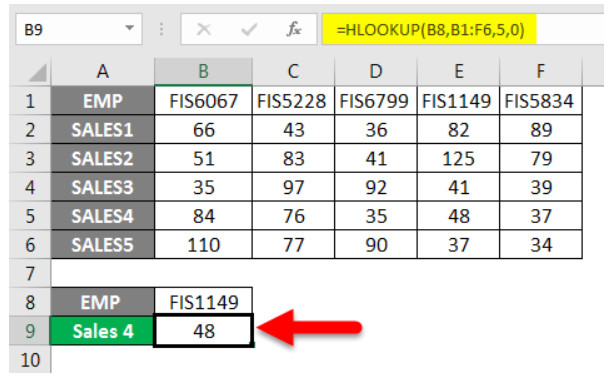
In this example:
- The lookup value (B8) represents the employee ID (FIS1149 in this case).
- B1:F6 is the range or table where the formula will search for the value.
- The row index (5) indicates the row containing the desired result.
- By setting the match type to 0, we ensure an exact match.
Example 5: Approximate Match
In certain scenarios, an approximate match might be more suitable. Let’s find out which city has a temperature closest to the value mentioned in cell B5, using an approximate match.

HLOOKUP Formula for the above example
=HLOOKUP(B4, B1:F2, 2, TRUE)
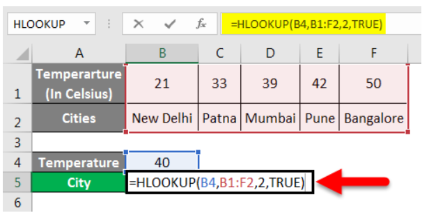
Press enter to get your results
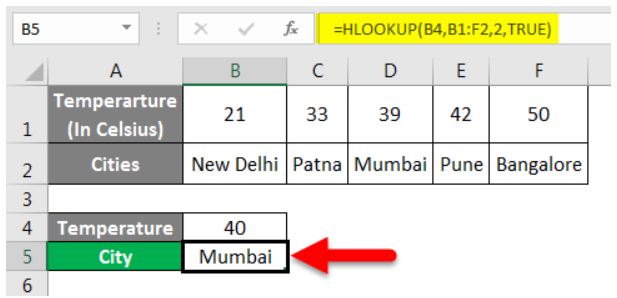
In this example:
- The lookup value (B4) represents the desired temperature.
- B1:F2 is the range or table where the formula will search for the value.
- The row index (2) indicates the row containing the desired result.
- By setting the match type to True, we allow for an approximate match within a specified range.
Example 6: Using Wildcards
Sometimes, we might not remember the exact name of a specific item. In such cases, we can use wildcards to match a part of the name. Let’s find the sales for an employee whose name starts with “Cat.”

HLOOKUP Formula
=HLOOKUP(“Cat*”, B1:G2, 2, 0)
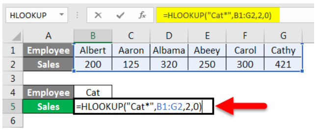
Ht the enter button for the results
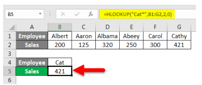
In this example:
- The lookup value (“Cat*”) represents the wildcard search term.
- B1:G2 is the range or table where the formula will search for the value.
- The row index (2) indicates the row containing the desired result.
- By setting the match type to 0, we ensure an exact match.
Conclusion
By harnessing the power of the HLOOKUP formula in Excel, you can efficiently retrieve values from horizontal sequences, simplifying data analysis and manipulation tasks. Remember to choose the appropriate match type, utilize wildcards when necessary, and explore the vast possibilities this formula offers. With practice, you’ll become an Excel master capable of conquering complex data challenges.

