As an essential tool for data management, Excel empowers users to organize, analyze, and present information in a structured and visually appealing manner. Panes, which divide the Excel window into separate sections, are often employed to simultaneously view different areas of a large worksheet or to freeze specific rows and columns for easy navigation.
However, there may come a time when you no longer require these panes, whether due to a change in your data analysis needs or simply to declutter your workspace. In this blog post, we will walk you through various methods to remove panes in Excel.
By the end, you will possess the knowledge and confidence to efficiently eliminate unwanted panes, optimizing your Excel experience and streamlining your workflow. So let’s dive right in and discover the step-by-step procedures for removing panes in Excel, ensuring that your spreadsheet work remains seamless and hassle-free!
Understanding Panes
Before diving into the methods of removing panes in Excel, it’s essential to have a clear understanding of what panes are and how they function within the software. Panes in Excel refer to the ability to split the worksheet into separate sections, allowing you to view different parts simultaneously.
This feature can be particularly useful when working with large datasets or comparing data from different areas of the worksheet. By splitting the worksheet into panes, you can freeze specific rows or columns, keeping them visible while scrolling through the rest of the worksheet.
This feature is commonly used to keep header information or key data visible at all times, providing easy reference points as you navigate through the data. Now that we have a better grasp of the concept of panes, let’s explore various methods to remove panes in Excel and return to a single-pane view.
How to Remove Panes in Excel: Step-by-Step Guide
Removing Panes Using the Ribbon
- Open the Excel workbook that contains the worksheet with panes.
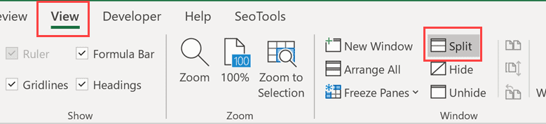
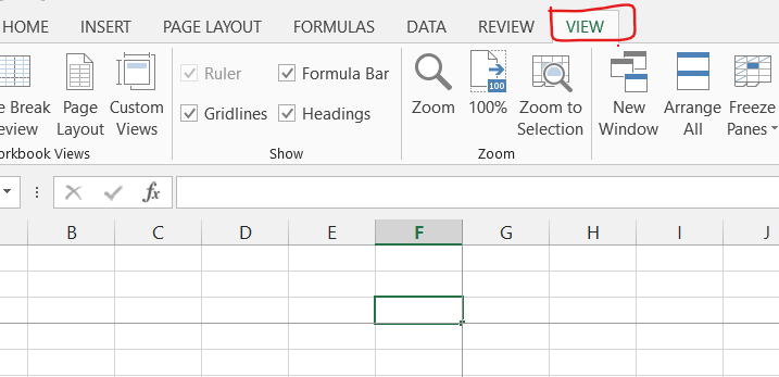
- Click on the “View” tab in the Excel ribbon.
- Locate the “Window” group and click on the “Split” button to toggle off the split panes. The split bars will disappear, and the worksheet will return to a single-pane view.
Removing Panes Using the Keyboard Shortcut
- Open the Excel workbook that contains the worksheet with panes.
- Press the “Alt” key on your keyboard to activate the ribbon.
- Press the “V” key to select the “View” tab.
- Press the “W” key to toggle off the split panes. The split bars will disappear, and the worksheet will return to a single-pane view.
Removing Panes Using the Context Menu
- Right-click on any cell within the worksheet that has panes.
- In the context menu that appears, select “Split” to remove the split panes and return to a single-pane view.
Removing Panes Using the Freeze Panes Option
- Open the Excel workbook that contains the worksheet with panes.
- Click on the cell below and to the right of the panes you want to remove. This will be the first cell that is not frozen or split.
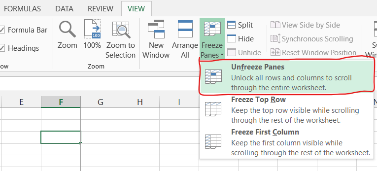
- Navigate to the “View” tab in the Excel ribbon.
- In the “Window” group, click on the “Freeze Panes” dropdown.
- Select “Unfreeze Panes” from the dropdown menu. The frozen or split panes will be removed, and the worksheet will return to a single-pane view.
Best Practices for Removing Panes in Excel
When removing panes in Excel, it’s important to keep in mind some best practices to ensure a smooth and efficient workflow. Here are a few tips to consider:
- Save your work before removing panes: It’s always a good idea to save your Excel workbook before making any changes. This way, you can easily revert to the previous version if needed.
- Understand the impact of removing panes: Removing panes will affect the layout of your worksheet. Make sure to review the contents and formatting of your worksheet after removing panes to ensure everything is displayed correctly.
- Utilize the “Zoom” feature: If removing panes causes the worksheet content to become too small or difficult to read, consider adjusting the zoom level in Excel. You can do this by clicking on the “View” tab and using the zoom options available.
Conclusion
In this article, we explored various methods to remove panes in Excel and return to a single-pane view. Whether you prefer using the ribbon, keyboard shortcuts, or the context menu, Excel offers multiple options to accomplish this task.
Additionally, we provided best practices to consider when removing panes and answered some frequently asked questions related to the topic. By following the step-by-step instructions and applying the tips mentioned, you can efficiently remove panes in Excel and enhance your spreadsheet workflow.