Comparing and matching data between two columns is a common task in Excel. Whether you want to find duplicate records, identify missing values, or compare lists, matching columns in Excel is essential.
In this comprehensive guide, you will learn 5 easy ways to compare and match two columns in Excel:
- Using IF formula
- With VLOOKUP and HLOOKUP
- Using Conditional Formatting
- Counting Matches and Differences
- Matching on multiple criteria
By mastering these techniques, you can quickly spot duplicates, differences, and similarities across any two data columns in Excel.
So let’s get started matching columns like a pro!
Quick Overview of 5 Ways to Match Columns in Excel
Here’s a quick summary of the various methods to match two columns in Excel:
- IF formula checks if two cells match, returning “Match” or “No Match”
- VLOOKUP matches vertically, HLOOKUP matches horizontally
- Conditional Formatting highlights duplicate or unique values
- COUNTIF and COUNTIFS count matching or different values
- Advanced formula with multiple IF conditions can match multiple criteria
Now let’s look at each of these column matching techniques in more detail with examples.
1. Match Columns Using IF Formula
A simple IF formula can compare two cells and output custom text if they match or not:
=IF(A2=B2,”Match”,”No Match”)
- Checks if Cell A2 = Cell B2
- Returns “Match” if true, “No Match” if false
To compare entire columns:
- Enter IF formula in Cell C2
- Fill down to additional rows with data
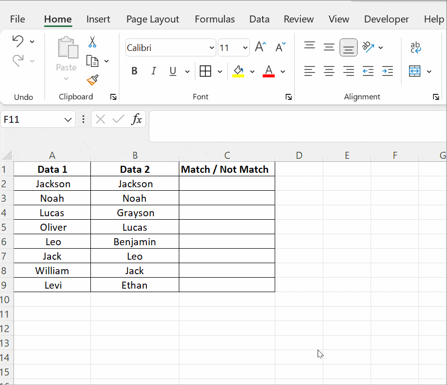
This quickly compares each row to highlight matches and differences.
You can also count matches and differences with COUNTIF:
=COUNTIF(C:C,”Match”) =COUNTIF(C:C,”No Match”)
2. Match Data Using the LOOKUP Function
The LOOKUP function is a valuable tool for searching for a specific value within a single row or column and retrieving a corresponding value from another row or column. Excel offers several variations of the lookup function, including HLOOKUP, VLOOKUP, and XLOOKUP. In this context, “H” and “V” denote horizontal and vertical, respectively, and the XLOOKUP function combines the features of both LOOKUP and VLOOKUP.
In the following example, we will focus on using the VLOOKUP() function to compare two columns in Excel effectively.
Scenario:
Column A contains a list of exams taken by a student, while column B comprises the subjects that the student has passed. Our objective is to create a result sheet containing a list of all subjects, with VLOOKUP() helping us in this process.
Here’s how you can apply the VLOOKUP() function in cell C2: =VLOOKUP(A2, $B$2:$B$5, 1, 0).

Now, to extend this comparison to all the cells below C2, simply drag the formula downwards. The result will appear in column C, with subjects that have been cleared and those that have not been cleared marked as #N/A.
3. Highlight Matching or Unique Values with Conditional Formatting
Conditional formatting lets you highlight matches or differences without formulas.
To highlight duplicates:
- Select columns to check
- Home > Conditional Formatting > Highlight Cells Rules > Duplicate Values
- Pick format to apply
To highlight unique values:
- Select columns to check
- Conditional Formatting > Highlight Cells Rules > Unique Values
- Pick format to apply

This visual format makes matches and differences easy to identify.
4. Count the Number of Matching or Different Values
You can get a count of matching and different values using COUNTIF or COUNTIFS:
Count matches:
=COUNTIF(C:C,”Match”)
Counts cells containing “Match”
Count differences:
=COUNTIF(C:C,”No Match”)
Counts cells containing “No Match”
Count with multiple criteria:
=COUNTIFS(C:C,”Match”,A:A,”x”)
Counts matches where column A = x
This gives statistics on matches and differences found.
5. Match Columns Based on Multiple Criteria
To match on multiple conditions, nest IF statements:
=IF(A2=B2, “Match”, “Mismatch”)

You can add more AND/OR conditions to match based on multiple criteria.
This allows matching only when all/any conditions are met.
Interactive Matching with Helper Columns
For a visual interactive approach:
- Add Result column with IF formula
- Toggle values in one column to see matches change
This allows for playing with scenarios and instantly seeing the matched output.
Top Tips for Matching Columns in Excel
Follow these tips for easy column matching:
- Use absolute references in formulas for copying
- Check for case-sensitive matches with EXACT
- Reference other sheets or books for advanced matching
- Filter data first to match only relevant records
- Use conditional formatting to visually identify matches
- Combine MATCH and INDEX to return actual values
- Dynamically count matches with COUNTIF as you go
- Rearrange data for vertical or horizontal lookup
Matching columns in Excel is crucial for analyzing and cleaning data. Master these techniques to compare data like an expert.
Conclusion
Whether you want to find duplicate data, identify missing values, check accuracy, or highlight differences, matching columns in Excel is essential. With these handy tools under your belt, you can match, compare, and analyze data across columns for better insights. So level up your Excel skills now with these 5 easy ways to match two columns like a pro.