Excel is a powerful tool for data analysis and organization, and its filtering capabilities allow users to easily sort and narrow down information. However, the AutoFilter arrows that appear when applying filters can sometimes clutter the spreadsheet and affect its overall visual appeal.
If you’re looking to hide those filter buttons in Excel and create a cleaner and more streamlined view of your data, you’re in the right place.
In this step-by-step guide, we will walk you through the process of hiding filter buttons in Excel, enabling you to maintain a visually appealing spreadsheet while still utilizing the filtering functionality. Let’s dive in and discover how you can achieve this effortlessly in Excel.
Understanding Filter Buttons in Excel
Filter buttons, also known as auto-filter buttons, are small drop-down arrows located next to the column headers in Excel. These buttons enable you to apply filters to a column, allowing you to display only the data that meets specific criteria.
By clicking on a filter button, you can choose from various filtering options, such as sorting in ascending or descending order, filtering by specific values, or applying custom filters.
Why Hide Filter Buttons?
Hiding filter buttons can be beneficial in several scenarios. It can help improve the visual appearance of your Excel worksheet by reducing clutter and creating a cleaner layout.
Additionally, hiding filter buttons can prevent accidental changes or modifications to the filtered data, ensuring data integrity. Moreover, if you are sharing your Excel file with others and want to restrict access to the filtering functionality, hiding filter buttons can serve as an effective security measure.
Hide Filter Buttons in Excel – A Step-by-Step Guide
To begin, we will utilize the advanced filter feature to filter data while keeping the AutoFilter arrows hidden. Let’s walk through the process step by step:

Step 1: Setting up the Criteria Values
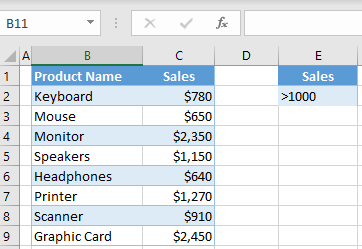
- First, consider the example where we have a table containing the “Product Name” and “Sales” columns.
- Create a separate table or range outside the filtering range to define your criteria values. In our case, we will use the heading name “Sales” and set the criteria value to be greater than 1000.
- This criteria range should be placed in cells E1:E2.
Step 2: Performing the Filter
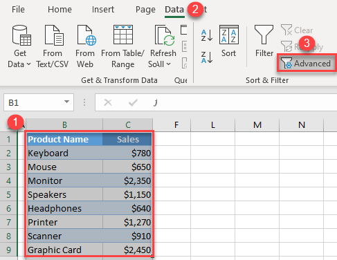
- Select the range of data that you want to filter. In our example, the range is B1:C9.
- On the Ribbon, navigate to the “Data” tab and click on the “Sort & Filter” button.
- From the drop-down menu, choose “Advanced” to open the Advanced Filter window.
Step 3: Configuring the Advanced Filter
- In the Advanced Filter window, you will see the option to specify the criteria range.
- Here, select the range E1:E2 that contains your criteria values.
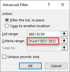
- Click on the “OK” button to apply the filter.
Step 4: Observing the Filtered Results
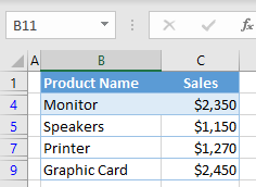
- After applying the advanced filter, you will notice that the filtered results appear just like they did with the standard filtering method.
- The only significant difference is the absence of the AutoFilter arrows in Row 1. This provides a cleaner and more streamlined view of your filtered data.
By following these simple steps, you can now filter your data effectively while keeping the AutoFilter arrows hidden. This approach not only allows you to maintain a visually appealing spreadsheet but also provides a seamless filtering experience.
Tips for Working with Hidden Filter Buttons
- Always make sure to document the steps you followed to hide filter buttons. This will help you remember the process and reproduce it if needed.
- When sharing an Excel file with hidden filter buttons, provide clear instructions to the users about the hidden functionality and how to unhide the buttons if necessary.
- Avoid using too many hidden filter buttons, as it may make it challenging to manage and maintain the worksheet.
- Regularly review and update your Excel files to ensure the hidden filter buttons are functioning as intended.
Conclusion
Now that you have learned how to hide filter buttons, you can take your Excel skills to the next level and create visually appealing and well-organized spreadsheets. Experiment with different filters and explore the various possibilities that Excel offers for data manipulation and analysis. With practice, you will become a master of Excel’s filtering features, allowing you to work more efficiently and present your data in a polished and professional manner.
Remember, Excel is a versatile tool, and continuously expanding your knowledge and skills will enable you to harness its full potential. Keep exploring, learning, and refining your Excel expertise. Stay tuned for more helpful tips and tricks to elevate your Excel proficiency. Happy filtering!