While a blank spreadsheet may be the picture of serenity, a lot of people find them daunting. All that emptiness is just begging to be filled with lists, tables, and calculations. However, if you’re not careful, your spreadsheet can quickly become a cluttered mess.
One way to help keep your spreadsheet tidy is to grey out unused cells. This way, you can focus on the cells that are actually being used and ignore the rest.
And if you ever need to use those empty cells, they’ll still be there waiting for you. So how do you grey out unused cells in Excel? That’s what we’re here to show you. In this detailed guide, we’ll walk you through the steps to do it the right way.
What Does “Grey Out” Mean In MS Excel?
In Excel, grey out refers to the process of making a cell uneducable. This can be useful if you want to prevent users from accidentally changing a cell’s value, or if you want to make sure that a certain value is entered into a cell before other calculations can be performed.
When you “grey out” something in Excel, it means you’re making it less visible by changing the color to a light grey. This is often used to de-emphasize certain cells or ranges that aren’t relevant at the moment. For example, let’s say you have a worksheet with a bunch of sales data for different regions.
You might want to “grey out” the cells for regions that aren’t currently active. That way, you can focus on the data that’s most relevant without getting distracted by the rest. There are a few different ways to grey out cells in Excel, but we’ll walk you through the one that’s easy to do so.
How to Grey Out Unused Cells in Excel – A Step-by-Step Guide
Whether you’re looking to grey out entire rows, columns, or just individual cells, we’ve got you covered. Follow along with this step-by-step guide and you’ll have your cells greyed out in no time.
Use Excel’s “Conditional Formatting” Feature
One of the easiest ways to grey out unused cells in Excel is by using the conditional formatting feature. This one allows you to apply formatting based on certain conditions that you specify. Here’s how to do it:
- Select the cells that you want to grey out.

- Click the “Conditional Formatting” button in the “Styles” group of the “Home” tab.

- Select “New Rule” from the drop-down menu.

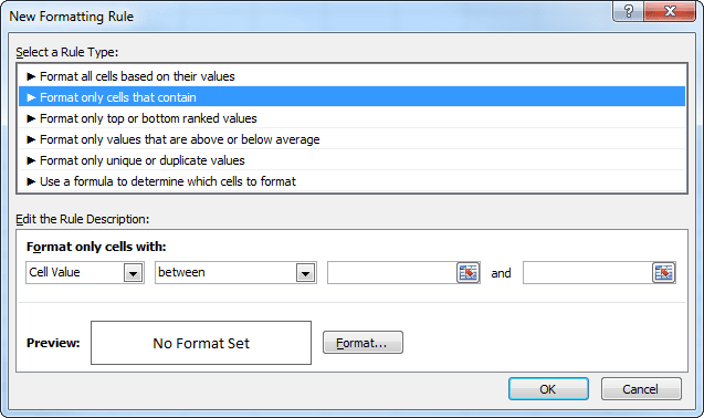
- In the “New Formatting Rule” window, select “Format only cells that contain” from the “Rule Type” drop-down menu.

- Then, select “(Your condition)” from the “Format only cells with” drop-down menu.

- Click the “Format” button to open the “Format Cells” window.

- Select the “Fill” tab and then choose a light grey color from the palette.

- Click “OK” to close the “Format Cells” window.

- Click “OK” again to close the “New Formatting Rule” window.

- Your selected cells should now be greyed out.
Verdict
That’s all there is to it! Now you can easily grey out any unused cells in your Excel sheet. We hope this little tip comes in handy for you and makes your data analysis just a bit easier. As always, if you have any questions or comments feel free to reach out to us – we love hearing from our readers!

