Excel, the ubiquitous spreadsheet software from Microsoft, is an invaluable tool for organizing, analyzing, and manipulating data. Whether you’re a seasoned data analyst, a financial whiz, a student managing academic records, or simply someone working with numbers, chances are you’ve relied on Excel to streamline your tasks.
While Excel offers an array of powerful features, one common challenge users often encounter is handling wide datasets where they need to scroll horizontally to view all the information. This is where freezing columns comes to the rescue! By freezing two columns, you can keep essential data in sight at all times, regardless of how far you navigate through your sheet.
In this blog post, we’ll take you through a step-by-step guide to freezing two columns, boosting your efficiency, and making Excel work even harder for you. So, buckle up and get ready to unravel the secrets of this time-saving technique, empowering you to tame unwieldy data and enhance your Excel expertise!
Understanding Excel’s Freeze Panes Feature
The Freeze Panes feature in Excel is a crucial tool that empowers users to lock rows and columns in position while navigating through a worksheet. By “freezing” specific areas, important data remains constantly visible, regardless of scrolling actions.
This functionality proves invaluable, especially when working with large datasets that extend beyond the screen’s visible area. By preserving headers, labels, or essential information, users can efficiently analyze and manipulate data without losing context.
The term “freezing” metaphorically captures the concept of locking these elements in place, akin to preserving them in time. Understanding the significance of the Freeze Panes feature sets the foundation for learning how to freeze two columns in Excel effectively, optimizing productivity and data analysis.
Freezing the First Two Columns
To freeze the first two columns in Excel, follow these simple steps:
Step 1: Open your Excel worksheet
Launch Microsoft Excel and open the worksheet you want to work with.
Step 2: Identify the columns to freeze
Determine which columns you want to freeze. In this case, we want to freeze the first two columns (A and B).
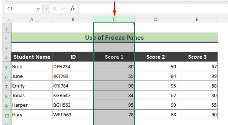
Step 3: Select the Column Next to the 2 Columns
Click on the column that lies to the right of the columns you wish to freeze. This ensures the frozen columns remain visible, and the rest of the worksheet can be scrolled horizontally.
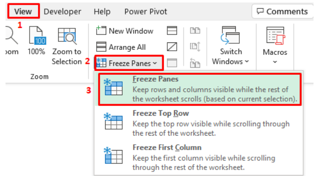
Step 4: Navigate to the “View” tab
Locate the “View” tab on the Excel toolbar. Click on it to reveal the View options.
Step 5: Freeze the columns
In the “View” tab, find the “Freeze Panes” dropdown menu. From the options, select “Freeze Panes.” Excel will then freeze the columns to the left of the selected cell.
Step 6: Verify the frozen columns
Scroll through the worksheet to ensure the first two columns remain fixed on the screen, providing you with easy access to the data as you explore the rest of the data.

Alternatives to Freezing Columns
While freezing columns is a valuable feature, it might not always be the best solution. There are alternative methods to enhance your data analysis experience:
Split Window View: Excel allows you to split the worksheet into multiple panes, each with its scroll bar. This feature enables you to view different sections of the same worksheet simultaneously.
Data Filters: Using Excel’s data filters can help you focus on specific data points without the need to freeze columns. Filters allow you to display only the information that meets certain criteria.
Hiding Columns: If freezing columns clutters your view, consider hiding unnecessary columns. Hidden columns can be easily unhidden when needed.
How to Unfreeze Panes in Excel
If you no longer need frozen columns, Excel provides a simple way to unfreeze them:
- Go to the “View” tab.
- Click on the “Freeze Panes” dropdown menu.
- Choose “Unfreeze Panes” from the options.
Enhancing Efficiency with Frozen Columns
Freezing columns in Excel significantly improves efficiency, especially when working with large datasets. With important data always visible, you can perform quick analyses and comparisons without losing sight of the context.
Utilizing Excel Productively
Excel offers a plethora of features that can expedite your tasks and optimize your productivity. By exploring its functionalities and keyboard shortcuts, you can become a proficient Excel user and handle complex spreadsheets with ease.
Conclusion
In conclusion, knowing how to freeze two columns in Excel can immensely improve your data analysis and overall productivity. The Freeze Panes feature allows you to keep vital information in sight while navigating through extensive worksheets.
However, it’s essential to consider alternative methods like Split Window View and data filters to suit specific tasks better. Embrace the power of Excel and become an efficient data handler, and you’ll witness a significant boost in your productivity.