The Chi-Square Test is a powerful statistical function in Excel that allows us to calculate the expected values from observed data sets. Excel, being a versatile tool for data analysis, provides not only visual representation but also advanced statistical functions.
These functions enable us to gain insights from datasets that may not be readily apparent through visual analysis alone. In this article, we will explore how to perform the Chi-Square Test using Excel and delve into some practical examples.
What is the Chi-Square Test?
The Chi-Square Test is primarily used to evaluate the validity of a hypothesis. The test helps us determine if the observed results are statistically significant or merely due to chance.
A statistically significant result indicates that we should reject the null hypothesis, which is a statement or assumption likely to be incorrect. The Chi-Square P-Value, a value between 0 and 1, plays a crucial role in this test. Typically, a Chi-Square P-Value below 0.05 leads to rejecting the null hypothesis.
Performing the Chi-Square Test in Excel
Let’s now explore how to conduct the Chi-Square Test in Excel with the help of practical examples.
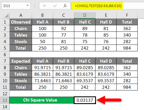
Step #1: Distributing Furniture
Suppose your company has a total of 10,000 pieces of furniture, and you want to determine the proportion of furniture distributed in four different halls.

To calculate the expected number of furniture items in each hall, follow the steps below:
- Calculate the expected value using the formula: Expected Value = Category Column Total x (Category Row Total / Total Sample Size). For instance, if we want to find the expected number of chairs in Hall A, the calculation would be as follows:Expected Number of Chairs in Hall A = 250 x (362 / 984)
- Calculate the difference using the formula: ((Observed Value – Expected Value)²) / Expected Value
- In the Chi-Square test, the value of ‘n’ is 2. For chairs in Hall A, the calculation would yield a value of 0.713928183. Repeat this step for each quantity, and the sum of these values will give us the test statistic. If each quantity is independent, this statistic will approximately follow a Chi-Squared distribution.
- Determine the degrees of freedom for each quantity using the formula: (number of rows – 1) x (number of columns – 1)
In this case, the degrees of freedom will be 6.
Calculate the Chi-Square P-Value for each quantity. The null hypothesis states that the location of the furniture is independent of the type of furniture.
- By summing all the Chi-Square P-Values, we can determine if the null hypothesis holds true. If the test statistic is excessively large for the given dataset, we reject the null hypothesis.
- For example, let’s assume the Chi-Square value for chairs is approximately 0.03. Based on our earlier discussion, we can conclude that this value leads to the rejection of the null hypothesis.
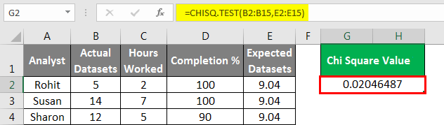
- To simplify this process, you can use the CHISQ.TEST Function in Excel, which directly provides the Chi-Square value and helps verify the assumption regarding the independence of furniture location and type.

Step #2: Calculating the P-Value
To calculate the p-value in Excel, follow these steps:
- Calculate the expected value, usually by obtaining the average or mean for normally distributed datasets. Refer to the previous example for more complex data scenarios.

- Organize your data into columns and select a blank cell where you want to display the results on the worksheet.
- Click the “Insert Function” button on the toolbar, and a pop-up window will appear.
- In the “Search for a Function” box, type “chi” and click “Go.” Select the “CHITEST” function from the list and click “OK.”
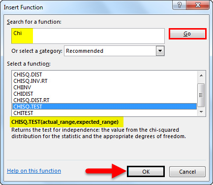
- Choose the observed and expected ranges and click “OK.”
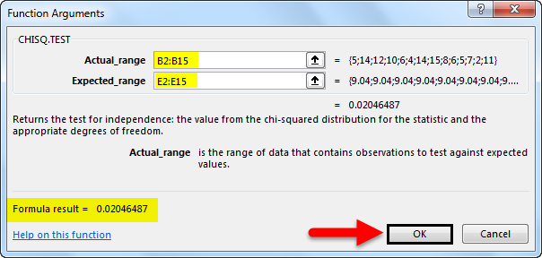
- The result will be displayed accordingly, providing you with the desired p-value.
Key Points to Remember
As you work with the Chi-Square Test in Excel, keep the following key points in mind:
- The CHISQ.TEST is not the only Chi Square function available in Excel. Various Chi-Square variations are accessible, depending on your level of statistical proficiency.
- You can directly type the CHISQ functions into a cell, similar to any other function in Excel. This approach saves time, particularly when you are familiar with the data ranges you are working with.
- When working with the CHISQ function, the dependability hinges on the organization, distribution, and preciseness of the hypotheses being evaluated.
- When using the Chi-Square Test for assessing significance, exercise caution and ensure careful analysis.
Conclusion
In conclusion, the Chi-Square Test in Excel is a valuable statistical tool that enables the analysis of observed and expected values in a dataset. By leveraging this function, you can make informed decisions based on statistically significant results.
Remember to employ the appropriate Chi Square function that suits your specific analytical requirements, and always ensure the accuracy of your hypotheses and data.