In the world of spreadsheet software, Microsoft Excel stands as an unrivaled titan, offering users a multitude of functions and features to simplify data manipulation and analysis. One such fundamental aspect of Excel is the ability to use parentheses.
Whether you’re a novice or a seasoned Excel user, mastering the art of adding parentheses can significantly enhance your spreadsheet skills. In this comprehensive guide, we’ll walk you through the step-by-step process of adding parentheses in Excel, unlocking new doors of efficiency and functionality.
Understanding the Importance of Parentheses in Excel
Before we delve into the mechanics of using parentheses in Excel, let’s take a closer look at why they hold such importance. Parentheses play a crucial role in maintaining a structured approach to calculations within Excel, ensuring that the order of operations remains clear and accurate.
When you’re working with formulas in Excel, especially those involving multiple calculations, parentheses act as powerful tools for grouping and prioritizing specific segments. Imagine you have a complex formula with various mathematical operations. Parentheses allow you to isolate certain portions of the formula, indicating that the enclosed calculations should be performed first. This ability to dictate the sequence of operations can significantly impact the final outcome.
In essence, parentheses act as a tool for organization and priority within Excel formulas. They enable you to avoid ambiguity and make your intentions explicit to the software, leading to more dependable and precise calculations. As we proceed, we’ll delve into the practical “how-to” of using parentheses effectively in your Excel formulas.
Step 1: Launch Microsoft Excel and Open Your Desired Workbook
To begin, launch Microsoft Excel on your computer. If you’re working on an existing project, open the workbook where you want to add parentheses. If you’re starting a new project, create a new workbook by clicking on “File” and selecting “New Workbook.”
Step 2: Select the Cell for Your Formula
Identify the cell where you intend to input your formula. Click on the cell to select it. This is where the result of your calculation will be displayed.
Step 3: Begin Your Formula with an Equal Sign (=)
In Excel, all formulas start with an equal sign (=). This signifies to Excel that you’re about to enter a calculation.
Step 4: Enter the Main Portion of Your Formula
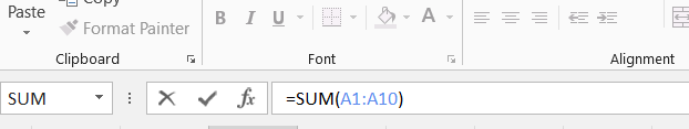
Now comes the exciting part—entering the actual formula. Type in the mathematical expression that you want Excel to evaluate. For example, if you’re calculating the total cost of items in cells A1 to A10, your formula might look like this:
=SUM(A1:A10)
Step 5: Introduce Parentheses for Grouping
Parentheses come into play when you need to group certain elements within your formula. Let’s say you want to add the values in cells A1 to A10 before multiplying the result by the value in cell B1. Your formula would appear as follows:
=(SUM(A1:A10)) * B1
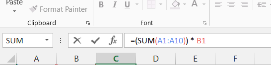
In this example, the parentheses around “SUM(A1:A10)” indicate that the addition should occur first, followed by multiplication.
Step 6: Nested Parentheses
Excel also allows you to nest parentheses, which means placing parentheses within parentheses. This advanced technique enables even more precise control over the order of operations. Suppose you want to divide the sum of cells A1 to A10 by the difference between cells B1 and B2, and then add the result to cell C1:
=((SUM(A1:A10)) / (B1 – B2)) + C1

Step 7: Closing Parentheses
Remember that each opening parenthesis must have a corresponding closing parenthesis. Excel uses this pairing to identify the scope of each operation. Ensure that you close your parentheses in the correct order to avoid errors in your formulas.
Step 8: Finalize and Evaluate Your Formula
Once you’ve entered your formula, double-check for any syntax errors or missing parentheses. When you’re confident in your input, press “Enter” to execute the calculation. Excel will process the formula according to the specified order of operations and display the result in the selected cell.
Conclusion
In conclusion, mastering the art of adding parentheses in Excel can significantly enhance your spreadsheet skills and streamline your data presentation. By following this comprehensive step-by-step guide, you’ve gained the ability to effectively organize calculations, prioritize formulas, and improve the clarity of your data.
Whether you’re a novice or an experienced Excel user, the power of parentheses can elevate your spreadsheet game and contribute to more accurate, visually appealing, and impactful data analysis. So go ahead, embrace this newfound knowledge, and excel in your Excel endeavors!