When working with data in Excel, it is often useful to visualize the relationship between two variables. One common way to do this is by adding a best-fit line, also known as a trendline, to a scatter plot.
A best-fit line helps us understand the overall trend and predict future values based on the existing data. In this article, we will explore different methods to add a best-fit line in Excel and evaluate its significance.
But before we dive into the methods of adding a best-fit line in Excel, let’s understand what it represents. A best-fit line is a straight line that represents the general pattern or trend in a scatter plot.
It shows the relationship between the independent variable (x-axis) and the dependent variable (y-axis). The best-fit line minimizes the overall distance between the line and the data points, giving us a good approximation of the relationship between the variables.
Adding the Best Fit Line in Excel: A Simple 3-Step Process
Now that you know what a best-fit line is and what its purpose is, let’s Learn how to effortlessly incorporate the Best Fit Line into your Excel charts with these easy steps:
Chart Selection: Start by selecting your desired chart.
Chart Elements: Access the “Chart Elements” button located on the right side of the chart. From there, follow one of the two options:
- Option 1: Check the “Trendline” box to insert the default Best Fit Line (linear).
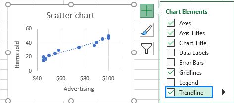
- Option 2: Click the arrow next to the “Trendline” box, explore the suggested types, and choose the most suitable one for your analysis.
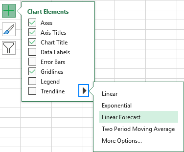
Customization: For further customization, access the “Trendline Options” tab within the “Format Trendline” pane. Explore the various trendline types available in Excel and select the one that aligns with your requirements. You can even choose to display the equation of the Best Fit Line directly on the chart.

Best Fit Line Integration in Excel 2010
For Excel 2010 users, here’s a tailored approach to adding the Best Fit Line to your charts:
Data Series Selection: Begin by clicking on the data series in the chart where you wish to incorporate the Best Fit Line.
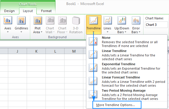
Layout Tab: Navigate to the “Layout” tab under “Chart Tools.”
Analysis Group: Locate the “Analysis” group within the “Layout” tab.
Trendline Selection: Click on the “Trendline” button and explore the predefined options or click “More Trendline Options…” to specify the Best Fit Line type that suits your data.
Unlocking the Potential: Multiple Lines of Best Fit in a Single Chart
Excel offers the flexibility to include multiple lines of best fit within a single chart. Here are two distinct scenarios:
1. Individual Lines of Best Fit for Each Data Series
To incorporate lines of best fit for multiple data series on a chart, follow these steps:
- Select the specific data points of interest (e.g., the blue data points).
- Right-click the selected data points and choose “Add Trendline” from the context menu.
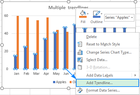
- Explore the “Trendline Options” tab and select the desired line type for each data series.
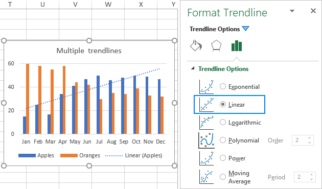
- Repeat the above steps for additional data series to ensure each has its own corresponding Best Fit Line.
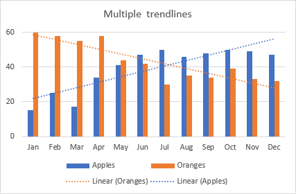
- Alternatively, you can use the “Chart Elements” button, select the arrow next to “Trendline,” and choose the appropriate Best Fit Line type for each data series.
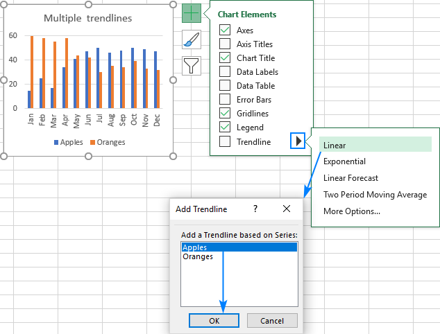
2. Multiple Best Fit Line Types for a Single Data Series
If you want to incorporate different lines of best-fit types within a single data series, follow these steps:
- Begin by adding the first Best Fit Line using the methods mentioned earlier.
- Right-click on the data series, select “Add Trendline” from the context menu and choose a different Best Fit Line type from the pane.
- Alternatively, utilize the “Chart Elements” button, select the arrow next to “Trendline,” and choose the desired Best Fit Line types to incorporate.
- Excel will display multiple lines of best fit in the chart, enabling you to set distinct colors for each line.

Customizing the Best Fit Line: Fine-Tuning Your Insights
To make your graphs even more visually appealing and comprehensible, you can customize the appearance of the Best Fit Line. Follow these steps to tailor its attributes:
- Right-click on the Best Fit Line and select “Format Trendline…” or double-click on the line to open the “Format Trendline” pane.
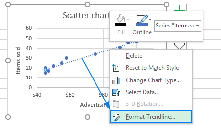
- Access the “Fill & Line” tab within the pane.
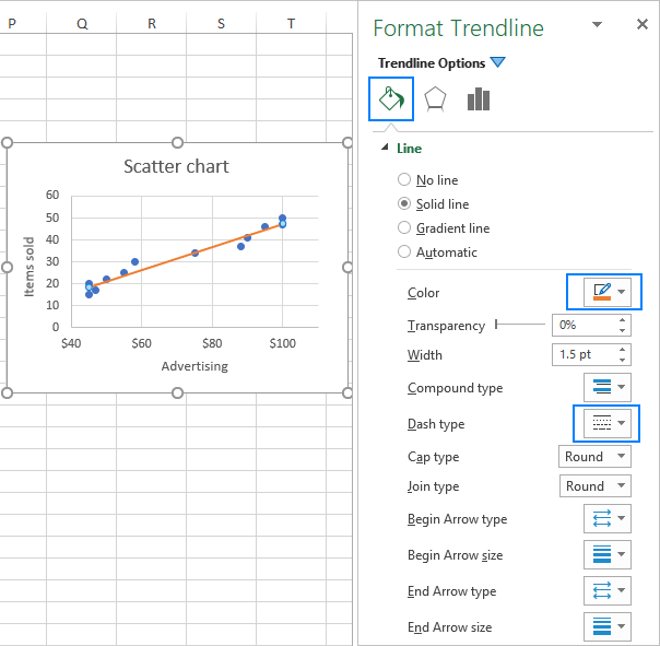
- Personalize the color, width, and dash type of the line to align with your preferences.
- For instance, you can transform a dashed line into a solid line to enhance clarity.
Extending Your Insights: Forecasting with Best Fit Line in Excel
Excel empowers you to project data trends beyond your existing dataset. Extend the reach of your Best Fit Line by following these simple instructions:
- Double-click on the Best Fit Line to open the “Format Trendline” pane.
- Navigate to the last tab, “Trendline Options.”
- In the “Forward” and/or “Backward” boxes under “Forecast,” input the desired values to extend the Best Fit Line accordingly.
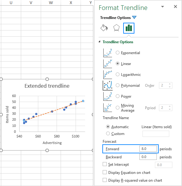
- Witness the enhanced predictive power of your Best Fit Line as it forecasts future trends.
Once you have added the Best Fit Line to your Excel chart, you can evaluate its significance and draw meaningful conclusions.
Wrap Up
In conclusion, adding a Best Fit Line to your Excel charts is a straightforward process that can greatly enhance your data analysis. By following a few simple steps, you can incorporate the Best Fit Line into your charts with ease.
Whether you choose the default linear trendline or explore different types based on your analysis needs, Excel provides customization options to tailor the trendline to your requirements. Furthermore, Excel allows for the inclusion of multiple lines of Best Fit, either for individual data series or within a single data series with different types.
By customizing the appearance of the trendline and utilizing forecasting capabilities, you can fine-tune your insights and project future trends. With the addition of the Best Fit Line, Excel empowers you to draw meaningful conclusions and unlock the full potential of your data analysis.

