This article will demystify and help you walk through the basics of Excel and make your journey of how to understand Microsoft Excel a lot simpler and enjoyable. Making your basics crystal clear is essential if you want to understand the advanced functionality of Excel.
So, let’s get started with the building blocks of Excel;
A Single Spreadsheet
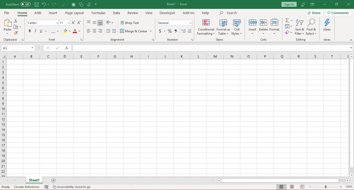
It is a single spreadsheet consisting of rows and columns. It is basically an element of the Excel Workbook. By default, the name of the first worksheet is “Sheet1”. So, a workbook is like an entire textbook, while a worksheet is a single page within that book.
A worksheet is in a tabular format consisting of rows and columns. Row numbers are placed vertically at the left side of the sheet and range from 1 to 1048576, whereas column headers are placed horizontally at the top of the sheet and range from A to XFD.
An intersection of a row and a column is called Cell and is identified with a combination of column headers and row numbers like A10 or C76.
Excel Workbook
In the query how to understand Microsoft excel you need to know about what an excel workbook is? It is the entire Excel file that contains one or more sheets. A simple Excel Workbook can be of a type – .xls or .xlsx. To create a new workbook, follow the steps below:
1. Open Excel and Click on File
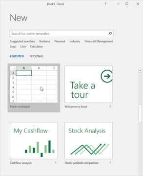
2. Click New, Under Featured, click on Blank workbook.
Ribbon
At the top of the Excel Window, there is a strip of buttons and icons called ribbon. It helps you navigate and choose from various commands of Excel.
An Excel Ribbon has five parts – Tabs, Groups, Command, Quick Access Toolbar, and Dialog launchers. The ribbon consists of various tabs like Home, Insert, Page Layout, Formulas, Data, Review, and View. Within each tab, there are several groups of commands.
For example
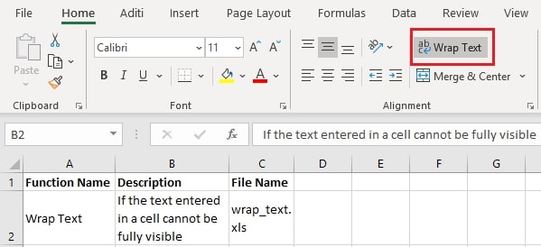
Home is a tab, and within the Home Tab, there is a group called “Alignment,” and under alignment, there is a command “Wrap Text.” The fourth component – A Quick Access Toolbar, is a customizable toolbar to add the most frequently used commands.
Lastly, a dialog launcher is a small downward pointing arrow in the bottom right of each group. It is used to open a dialog box that can be used to input information and make choices about different aspects of the current worksheet or its content.

Entering Data In Excel
Now that we have covered the basic terminology used in Excel, we will shift our focus onto entering information or functions in Excel. To enter data in Excel, simply select a cell and start typing. The text will appear on the Cell as well as on the formula bar at the top.
After entering the information, press Enter to submit the data and move to the Cell below or press tab to submit the data and move to the Cell on the right. To enter data on a new line within a cell, i.e., insert a line break, press Alt + Enter.
Types of data in excel
The three main types of data are Text, Number, and Formulas.
Text is mainly used to provide headings to tables/columns, write descriptions, etc., and contain letters, numbers, special characters. It is by default aligned to the left side of the Cell. Note: To enter a numerical value or formula as a text, type an apostrophe before it.
The number is used for calculations, and these are aligned towards the right side of the Cell. This type of data includes integers, decimals, percentages, currency, accounting, etc. To enter a date in Excel, type the date in the default format mm/dd/yyyy or whichever format is selected for that Cell. To change the format, simply press Ctrl + 1, then in the dialog box, select a date and select the appropriate format. Note: Dates and Time are also stored as numbers in Excel. January 1, 1900, is stored as number 1, and January 2, 1900, is stored as number 2.
To convert a text to a number, simply select the Cell and click on the small down arrow next to “General” under Home Tab and Select “Number.” Data will be converted to data with two decimal points.

You can increase or increase the decimal points using the icons under the number section of the Home tab again.

Formulas are mathematical equations that direct Excel to perform calculations. Each formula has a specific syntax that users must follow to make that function work. It uses hard-coded numbers and values in other cells to do calculations.
Examples are =32*(12+10) or =A2*B4 or =A2*(12+C4)
* Several custom number formats can be applied to the data in Excel. Let’s look at some of the examples below:
You can convert a number to a specific currency by selecting the Cell and then click on the small arrow next to the “$” icon under the Number section in the Home tab. From the dropdown list, select the desired currency.

For further customization, press Ctrl + 1, and in the dialog box, select “Currency.” From here, you can choose the currency of the symbol dropdown list, increase or decrease the decimal point and choose the formatting to negative values. A sample of your selection will also be displayed in the box.

* To convert a number into a percentage, simply press the “%” icon under the Home tab’s Number section. This will multiply the number by 100 and add a percentage sign to the display.

* To convert a number into accounting format, simply select Accounting from the dropdown in the number section. This will add the $ sign and two decimal places.

* To apply comma style, simply press the “icon under the Number section in the Home tab. This will add commas to large numbers and two decimal places (so 1000 becomes 1,000.00).
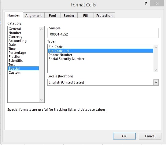
* To convert a number to Zipcode +4, Press Ctrl + 1, and under category select “Special.” This will convert the number to the pattern 00000-0000. Other options like social security numbers and phone numbers are also available in the same dialog box.
* If you want to add units to a number, you can do that using Custom Formatting. For example, you want figures in Millions in a table, and you want the word “Million” written next to the number with a $ dollar sign. (Convert 76 to $76 Million). To do that, press Ctrl + 1 and select Custom, and in the Type field, write $General” Million.” It will make the data look like text, but they are still a number.
* To add Color to your number type, go to Custom in Format Cell dialog box. Write color name enclosed in square brackets before the number format. If the current formatting is $#,##0, to add blue color the format will now be [blue]$#,##0.
Writing A Formula In Excel
To write a formula, begin with an = or + sign and use numbers or cell references in order to indicate which values are to be used in the calculation. Follow the steps below:
· Type = or +
· Enter cell references like A12 or F8
· Enter an operator like +, -, * or /
· Enter the second cell reference. Continue if necessary
· Hit Enter
Consider an example where there is a list of sales for 12 months, and total annual sales need to be calculated. This can be done using an excel formula.
There are two ways of doing it – How to understand Microsoft excel; a thought that triggers you to find more and more.
1. Create a summation formula where you add in all the numbers by typing them. Example =1787092+2467847+…….+2359196. Even though this formula will give you a correct answer, it will not be dynamic. This formula needs to be changed each time there is a change in the set of monthly sale values.
2. Create a formula that sums the value using cell addresses. Instead of inserting the number, we will give the cell reference that contains the number. Example: =SUM(B2:B13)
With this formula, the values that are inserted in the Cell will be used for calculation, making the formula dynamic.
In this second example below, we need to calculate fixed costs per unit. We have the total fixed cost entered in cell B2 and the number of units in cell B3. The result should be displayed in cell B4.
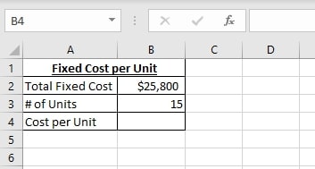
So, we will select cell B4 and write the formula =B2/B3 to get the amount of fixed cost per unit.
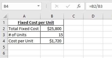
After creating this formula, even if you change the value in cell B2 or B3, the result in cell B4 will be updated automatically based on the new values.
Note: You can see that even though the result, i.e., $1720, is shown in cell B4, the formula, i.e., =B2/B3 is visible on the formula bar. You can even edit the formula directly from the formula bar.
In this example, we have used the formula to perform division; we can add, subtract or multiply the same way by simply changing the plus division to an appropriate operator in the formula.
The operator follows a default order in which the calculation occurs. The order of operators is as follows:
1. Parenthesis
2. Exponential
3. Multiplication and Division
4. Addition and Subtraction
So, if we use this formula =6+7*2, Excel will first multiply seven by 2, and then the result, i.e., 14, is added to 6. The result will then be 20.
For more information on formulas, click here<<link to Excel Formulas article>>
Format Data As Table
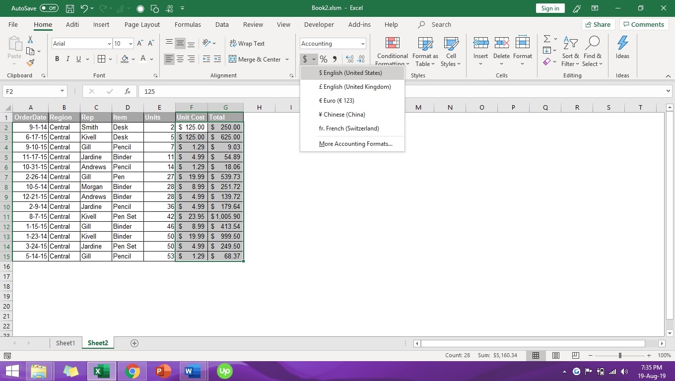
If we have a list of the information entered in Excel and want to format it as a table, we should follow the steps below:
* Click on any cell in the table and press Ctrl + A to select the entire table.
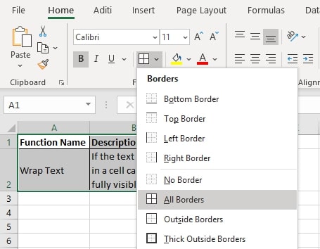
* To apply borders, Go to Home Tab > Under Font Group, Click on Borders icon > From the dropdown Select All.
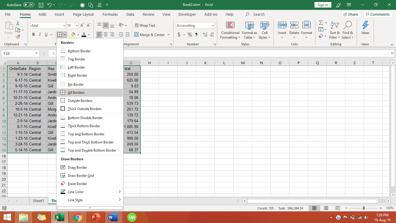
* Select the Headers of the table, and under Home Tab and Font Group, Select B (to make the header bold), fill color grey, and change the font color to white.
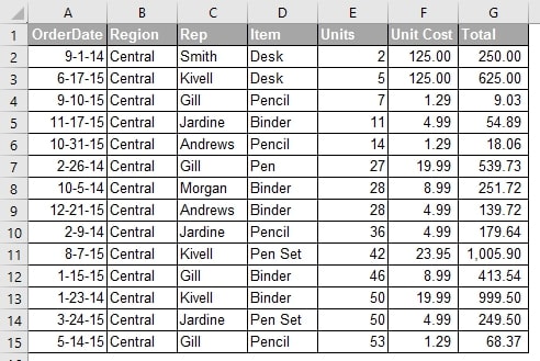
* Select Column F and G and change number formatting to currency. Go to Home Tab> Under Number Group > Click on the Dollar Sign > Select the appropriate currency.
Press Alt + W + V+ G to remove gridlines and your table with formatting is ready!
Formatting In Excel
The main goal of an Excel Worksheet is to make the data presentable, attractive and to be able to understand the data quickly. All this can be done using Excel formatting! The points below will guide you with the different ways of formatting the content:
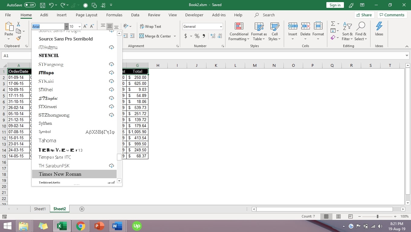
* Change Font – By default, the Font is set to Calibri. To change the Font, go to Home Tab > Click on the arrow next to the Font Command > Select the appropriate Font. If you hover on the different options in the dropdown, a live preview of the same will be visible.
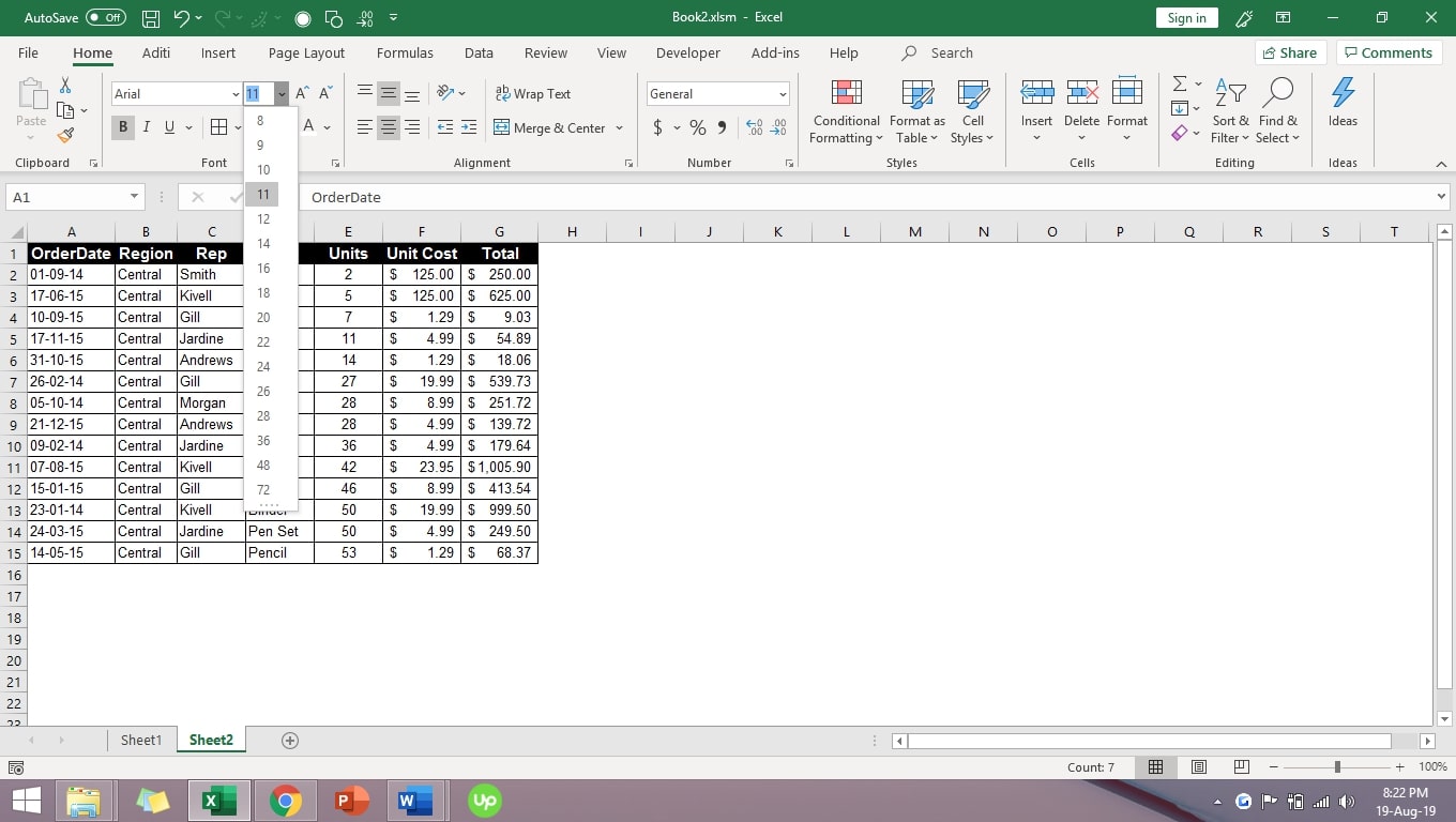
* Change Font Size – To change the font size, go to Home Tab > Click on the arrow next to the Font Size Command > Select the appropriate Font Size. You can click on either “Increase Font Size” or “Decrease Font Size” to change the size.
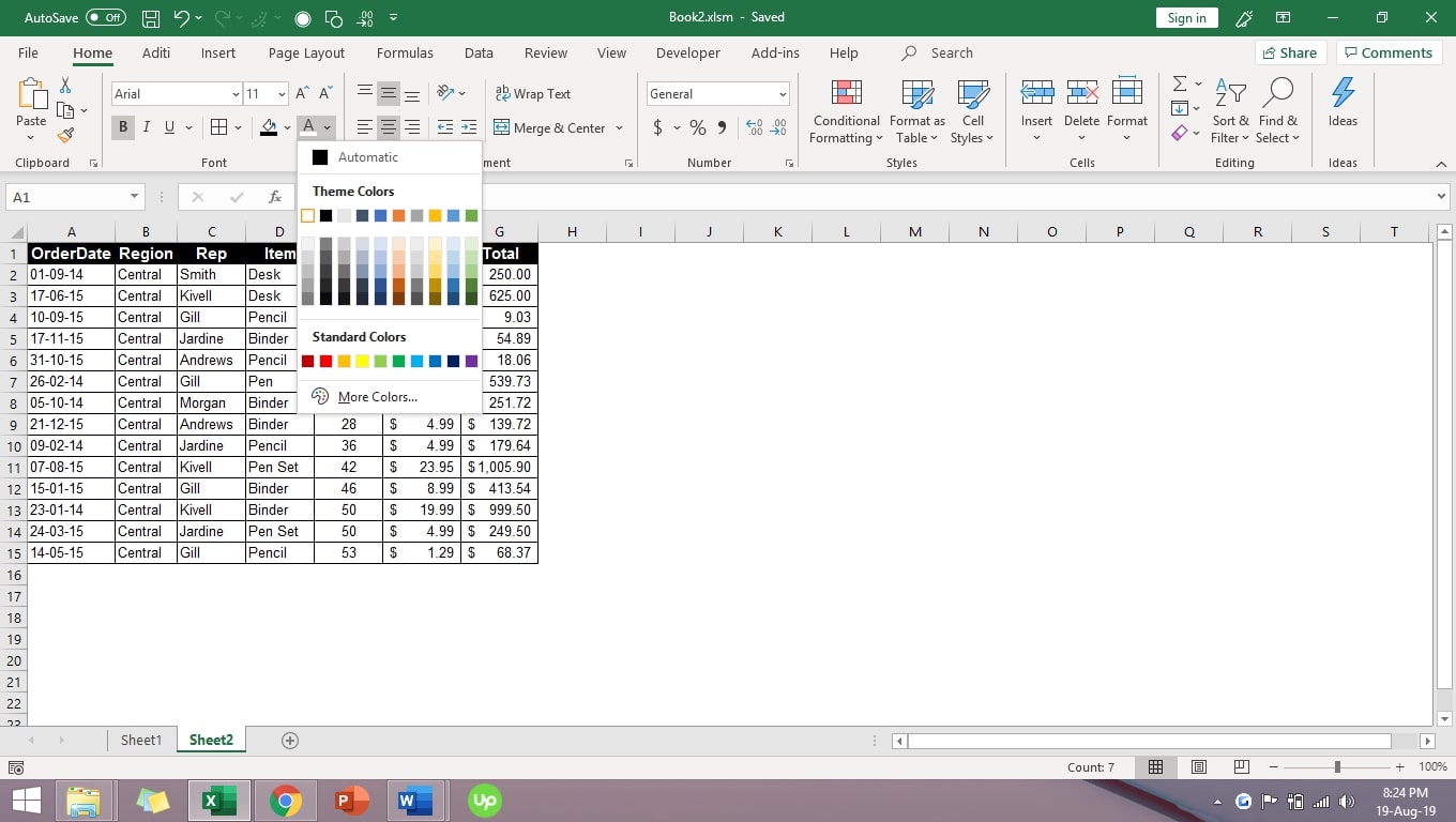
* Change Font Color – To change the font color, go to Home Tab > Click on the arrow next to the Font color Command > Select the appropriate Font color.
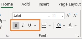
* Use Bold, Italics, Underline – Select the Cell where you want to apply the formatting. Press Ctrl + B to make text bold, Ctrl + I to make it italics, and Ctrl + U to make it underlined. Or else, you can simply click on “B,” “I,” or “U” symbols under Home Tab.
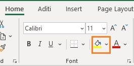
* Change cell color – Select Cell> Click on Home Tab > Click on the arrow next to Fill Color> Pick the Color you want. Or simply press Alt + H + H and pick the color you want.
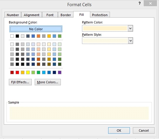
* Apply pattern – Select cell > Click on Home Tab > Click on Format Cells dialog launcher > Under Fill Tab > Select Pattern Color and Pattern Style.
* Change Horizontal and Vertical Alignment – Select Cell > Under Home Tab > Select Top, Middle, or Bottom alignment to change vertical alignment and Select Left, Middle, or Right Alignment to change horizontal alignment.


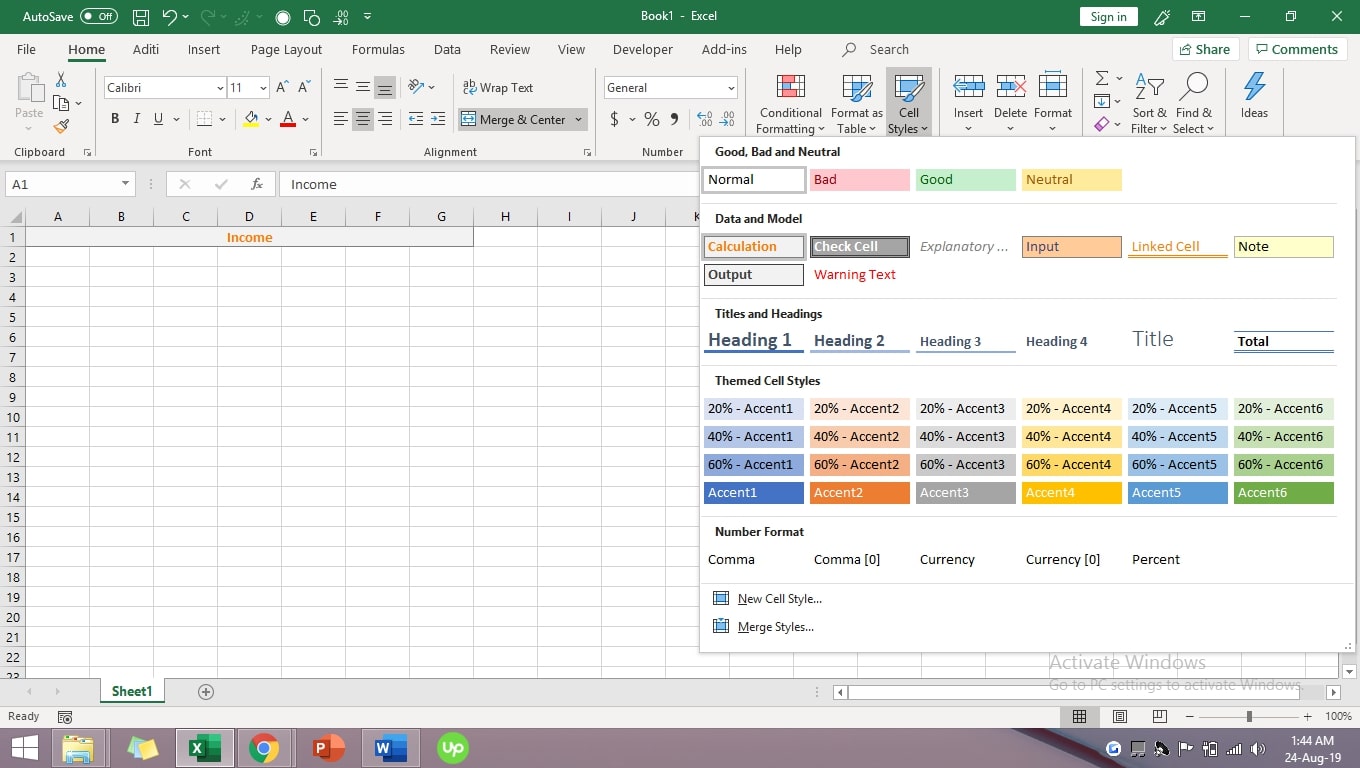
* Apply cell style – Select the Cell> Home tab > Click on cell style > Choose the desired style from the dropdown menu. Note: Once you select a cell style, all existing formatting except text alignment will be replaced.
* Wrap Text – If the text entered in a cell cannot be fully visible in a single line, we can select the Wrap Text function from Home Tab to make the data fit properly.
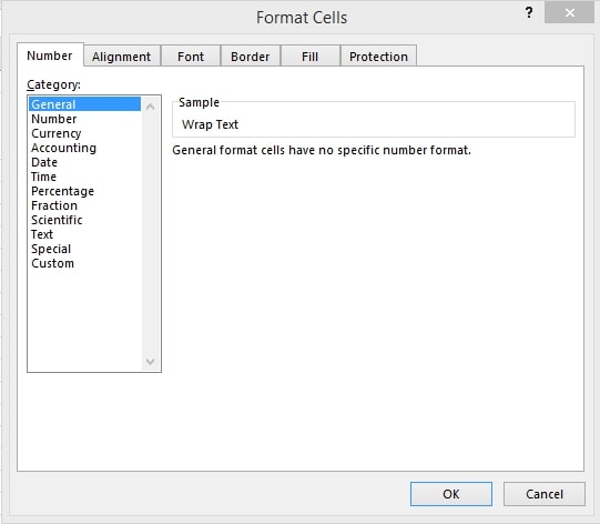
* Apply Number Formats – Under Home Tab > Click on the dialog box launcher; it will open the Format Cells dialog box where a complete list of number formats is available on the Number tab. You can select the desired format from various options, including numbers, dates, times, fractions, percentages, and other numeric values.
- Note: You can press Ctrl + 1 to open the Format Cell Dialog box.
- Note: Excel will sometimes change number formats automatically based on the data entered.
* Add Borders – To add borders, select the Cell and click on the borders icon under Home Tab. Select the appropriate border line and Color.
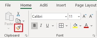
* Format Painter – To copy-paste formatting from one cell to another, simply select the Cell with formatting and click on the format painter icon in Home Tab and then click on the Cell where you want to paste the formatting.
Note – Once you click on the format painter icon, the arrow will be replaced with the format painter icon.
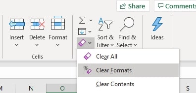
* Clear Formatting – To clear formatting in a cell, Select the Cell> Go to the Home tab > Go to the Editing group > Click on the arrow next to the Clear button > Select Clear Formats.
Printing Work Sheet In Excel
Now that your data is ready, you will need to print it. So, let’s move to the process of how to print a worksheet and the print setting available in Microsoft Excel.
The following points will guide you through the same:
* To print a worksheet, click on File tab > Click on Print. In the dialog box, we will be able to see a preview of the page that will be printed, and we can click on the big Print button to start printing.
Note: At the bottom of the dialog box, click on the previous or next button to preview other pages.
* To print multiple pages, hold down CTRL + click the name of each workbook to print, and then click Print.
* To print multiple copies, increase the number of copies from 1 to the desired number. You can also select collated or uncollated option from the dropdown. Note: Collated prints all pages of the 1st copy and then 2nd and so on whereas uncollated prints all copies of 1st page, then 2nd page, etc.
* To print only the active worksheet, click on “Print Active Sheet” from the dropdown under the settings option.

* Page orientation can also be changed (landscape or portrait) from the dropdown available.

* To adjust page margins, either select from the pre-defined options (Normal, Wide, or Narrow) Or click the ‘Show Margins’ icon at the bottom right of the window. Now you can drag the lines to change the page margins manually.

* If the entire table needs to be printed on 1 page, it can be done by selecting the “Fit Sheet on One Page” option from the scaling dropdown list. Other options available are “Fit All Columns on One Page” and “Fit.

* To set a print area, select the cells you want to print > go to Page Layout > Click on Print Area > Select Set Print Area.

Save An Excel File
To save an Excel file, click the Save icon in the top left of Excel or simply press Ctrl + S. A Save As dialog box will open; on the left panel, click on “Save As.” Under Save As, you can see four items: OneDrive, This PC, Add a Place and Browse. By default, the “This PC” option is selected, and your file will be saved in “My documents.”
If you want your file to be saved in the My Documents folder, type a file name and click on Save. Otherwise, click on the “More options…” link, select the desired folder, give a file name, and click on the Save icon.
Below The File Name Box
There is a dropdown from which you can select the file type like.xlsx or. xlsm etc.
In this article, we have tried to cover the basics of what Excel can do. Excel has many functions and formulas that can help you automate your work and make you faster and more efficient in Excel.
Follow us for more articles and tutorials to understand Microsoft Excel!

