Finding the p-value in Excel is a crucial task in statistical analysis. Whether you’re working on a research project or analyzing data, understanding how to calculate p-values is essential. In this article, we will explore two methods to find the p-value in Excel: using the T-Test function and the Data Analysis tool. Let’s dive right into it.
What is a P Value?
Before we delve into the intricacies of finding p values in Excel, let’s start with the basics. A p-value, short for “probability value,” is a statistical measure that helps determine the significance of a result in a hypothesis test. It quantifies the probability of observing a test statistic as extreme as the one computed from the sample data, assuming that the null hypothesis is true. In simpler terms, it tells us whether the observed data is statistically significant or merely a product of chance.
Why Are P Values Important?
Understanding p values is essential because they play a fundamental role in hypothesis testing and statistical analysis. When conducting experiments or analyzing data, researchers and analysts use p values to make informed decisions. A low p-value (typically less than 0.05) indicates strong evidence against the null hypothesis, suggesting that the observed results are unlikely to be due to random chance. On the other hand, a high p-value suggests that the data is consistent with the null hypothesis, meaning the results are not statistically significant.
Calculating P Values in Excel
Now that we’ve established the importance of p values, let’s get into the nitty-gritty of how to find them in Excel.
Method 1: Calculating P-Values with T-Test
The T-Test function is a powerful tool for evaluating the significance of data. Follow these step-by-step instructions to calculate the p-value using this method.
- Open Your Excel Document: Start by opening the Excel document you want to work with or create a new one. Ensure that you already have data in the workbook.
- Select a Cell: Choose any cell outside your data set. In this cell, input the following formula: =T.TEST(.
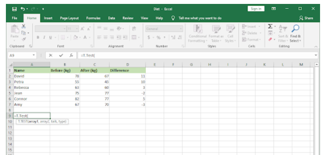
- Set the First Argument: Specify the first argument, which should be the entire data column you want to analyze, for instance, the “Before (kg)” column. The formula will automatically adjust to include the cell references.
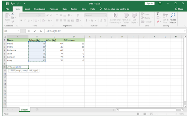
- Select the Second Argument: Add a comma (,) and choose the second argument, which is typically the “After (kg)” column in your data.

- Choose Distribution Type: Add another comma (,) and double-click on “One-tailed” from the options.

- Select Paired Data: Add one more comma (,) and double-click on “Paired.”

- Complete the Formula: All the necessary elements are now selected. Close the bracket with ), and then press Enter.

- View the P-Value: The selected cell will display the p-value.
So, what does this p-value mean? In our example, a low p-value suggests that the test didn’t result in significant weight loss. However, it’s important to note that this doesn’t prove the null hypothesis is correct; it merely means it hasn’t been disproven.
Method 2: Using Data Analysis to Find P-Values
The Data Analysis tool in Excel provides various ways to manipulate and analyze data, including finding p-values. Follow the instructions below.
- Open Your Excel Document: Open the Excel document you want to work with or create a new one with the required data.
- Access Data Analysis: Switch to the “Data” tab in the ribbon header interface, and click on “Data Analysis” from the “Analysis” group.

- Enable Data Analysis (if needed): If you don’t see the “Data Analysis” option, go to “File,” then “Options,” and select “Add-ins.” Click on the “Go” button, choose “Analysis ToolPak,” and click “OK.” The option will now appear in your ribbon.

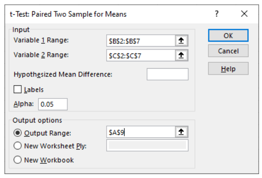
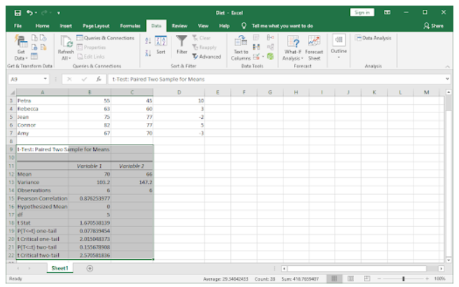
- Select Analysis Type: In the pop-up window, scroll down and choose “t-Test: Paired Two Sample for Means.” Click “OK.”

- Enter Arguments: Enter your arguments, ensuring you use a “$” symbol before each cell reference. For instance, your setup should resemble the example provided.
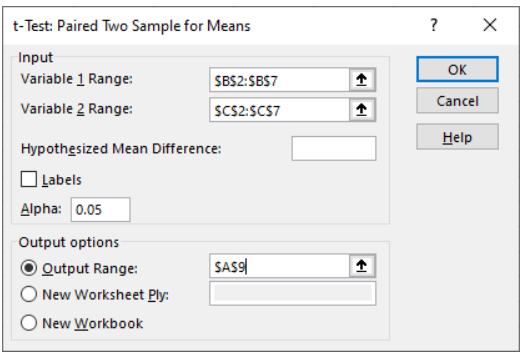
- Set Alpha Level: Leave the “Alpha” text box at the default value, which is typically 0.05.
- Specify Output Range: Choose the “Output Range” option and designate the cell where you want the p-value to appear, such as “A9.”
The final table generated will contain various calculations, including the p-value result, which can provide valuable insights into your data.
Conclusion
In conclusion, understanding how to find the p-value in Excel is a valuable skill for anyone working with data analysis. Whether you prefer the T-Test function or the Data Analysis tool, these methods empower you to make informed decisions based on statistical significance. So, choose the method that suits your project and skill level and start making data-driven conclusions.