Adding color to spreadsheets can be a highly effective way to visualize and analyze data in Excel. Color coding allows you to highlight important points, categorize data, spot trends, and simply make your spreadsheets easier on the eyes. Whether you’re looking to color code a handful of cells or entire sheets, Excel provides all the tools you need to quickly assign colors and transform plain, black-and-white workbooks into attractive, colorful documents.
Among its myriad features, color coding is a gem that can significantly enhance data visualization and interpretation. In this comprehensive guide, we will delve into the intricacies of how to color code in Excel. By the end of this article, you’ll have the expertise to wield Excel’s color coding capabilities with finesse, making your data come to life and stand out from the rest.
Why Color Coding Matters
Before we dive into the nitty-gritty of Excel’s color coding, let’s explore why it’s essential. In today’s fast-paced world, information overload is a common challenge. Whether you’re managing sales figures, tracking project deadlines, or analyzing survey results, Excel’s grids and columns can quickly become overwhelming.
Color coding offers a visual solution to this problem. By assigning specific colors to data points or categories, you can create a visual hierarchy that instantly conveys information. This visual hierarchy allows your brain to process and prioritize data swiftly, making it easier to spot trends, outliers, and key insights.
Steps to Color Code in Excel
Setting the Stage: Data Preparation
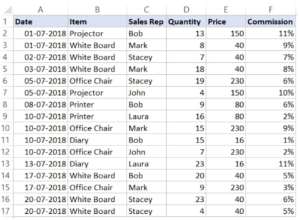
Before we embark on our color coding journey, it’s essential to ensure that your data is well-organized. Let’s assume you have an Excel worksheet containing a sales roster with details of purchases made at a store over the year. To get started, follow these steps:
Step 1: Organize Your Data
Begin by collecting your data and organizing it into well-labeled columns within your Excel worksheet. Each column should represent a specific attribute, such as customer names, product names, sales representatives, and purchase dates. This structured approach will lay the foundation for efficient color coding.
Step 2: Define Your Objective
In our scenario, let’s say our goal is to highlight all the sales records associated with a Sales Representative named “Bob.” Having a clear objective is crucial as it guides the entire color coding process.
The Magic of Conditional Formatting
Now that we have our data in place let’s dive into the fascinating world of Excel’s conditional formatting. Follow these steps to apply color coding based on matching values within the cells:
Step 3: Select Your Data
Highlight the entire dataset in your worksheet, which, in our example, would be the range A2:F17.
Step 4: Navigate to the “Conditional Formatting” Menu
Locate the “Home” tab on the top left corner of your Excel worksheet.

In the “Styles” group, you’ll find the “Conditional Formatting” option.

Step 5: Create a New Rule
Click on “Conditional Formatting” and select “New Rule.”

This action will open a ‘New Formatting Rule’ fly-out.
Step 6: Use Formulas to Determine Formatting
In the ‘New Formatting Rule’ fly-out, choose the option to “Use formulas to determine which cells to format.”

Step 7: Set Your Formula
In the formula dialogue box, input the following formula:
=$C2=”Bob”

This formula tells Excel to highlight the cells where the value in column C matches “Bob.”
Step 8: Define Your Formatting
Now, click on the ‘Format’ icon to specify the Excel color you want to use for highlighting.

Step 9: Choose Your Color
In the dialog box that appears, select the desired Excel color for highlighting. This color will be applied to rows where the Sales Representative is “Bob.”

Step 10: Apply and Review
Click “OK” to confirm your formatting choices. Excel will now highlight every row where Sales Rep “Bob” is located with the specified Excel color.

Best Practices for Effective Color Coding
While color coding can be a potent tool, it’s crucial to use it judiciously. Here are some best practices to keep in mind:
1. Choose a Meaningful Color Scheme: Select colors that convey meaning and are easily distinguishable. Avoid using colors that might confuse or mislead your audience.
2. Maintain Consistency: If you’re using color coding across multiple sheets or reports, ensure consistency in your color choices. This helps users understand and interpret the data consistently.
3. Provide a Legend: When sharing color-coded data with others, include a legend that explains the color associations. This ensures that everyone interpreting the data understands the meaning behind the colors.
Conclusion
In conclusion, mastering the art of color coding in Excel opens up a world of possibilities for data analysis and visualization. Whether you’re managing sales data, tracking project progress, or monitoring inventory levels, this technique can help you spot trends, outliers, and critical information at a glance.
With Excel’s conditional formatting, you can transform your raw data into a visually appealing and informative masterpiece. So, the next time you’re working with Excel, remember the power of color coding and how it can make your data come alive. Don’t just crunch numbers—let them tell a colorful story with Excel’s conditional formatting. Your journey toward data mastery has just taken a vibrant and insightful turn.