Understanding the relationship between two variables is a common task in statistical analysis. The correlation coefficient is a simple numeric measure that indicates both the strength and direction of the linear relationship between two variables. Excel makes it easy to find the correlation coefficient between two data sets. Here’s a step-by-step guide on how to find the correlation coefficient in Excel.
What is the Correlation Coefficient?
The correlation coefficient (r) measures the strength and direction of the linear relationship between two variables. Its values range from -1 to 1, with:
- -1 indicating a perfect negative correlation
- 0 indicating no correlation
- 1 indicating a perfect positive correlation
The closer the correlation coefficient is to -1 or 1, the stronger the correlation between the variables. The sign indicates whether the variables are positively related or negatively related.
When to Use the Correlation Coefficient
Finding the correlation coefficient is useful when you want to:
- Determine if two variables are related
- Assess the strength and direction of a linear relationship
- Make predictions about one variable based on the other
- Evaluate causal relationships between variables
For example, you may calculate the correlation between study time and test scores to see if more study time leads to higher scores. Or the correlation between age and health care costs to assess if age predicts higher costs.
How to Find the Correlation Coefficient in Excel
Finding the correlation coefficient in Excel is simple when you use the CORREL function. Follow these steps:
Step 1: Enter the Data
- Arrange your data with x-values in one column and y-values in the adjacent column.
- Input at least two data points of each variable. More data points will increase accuracy.
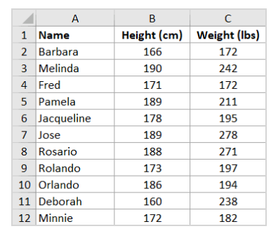
In our case we have arranged our values as Height and Weight:
Step 2: Click the Formulas Tab
- Select the Formulas tab in the top menu.

Step 3: Click Insert Function
- Click the Insert Function button (fx) on the left side of the formula bar.

Step 4: Search for CORREL
- Search for “CORREL” and double-click it to select.

Step 5: Select the Data Ranges
- For Array1, select the range of cells containing the x-values.
- For Array2, select the range of cells containing the y-values.

Step 6: Press Enter
- The correlation coefficient will be calculated and displayed in the cell.

Interpreting the Correlation Coefficient
Once you have the correlation coefficient, interpret its sign and value:
- Positive r values indicate a positive relationship – as x increases, y tends to increase.
- Negative r values indicate a negative or inverse relationship – as x increases, y tends to decrease.
- r values near zero indicate little or no linear correlation.
- An r value of 1 represents a perfect positive correlation, meaning the data points fall on a straight line with positive slope.
- An r value of -1 represents a perfect negative correlation, with the points falling on a straight line with negative slope.
- Larger absolute r values (ignoring the sign) indicate a stronger linear association.
Correlation Does Not Imply Causation
While the correlation coefficient measures the strength of the linear relationship between variables, it does not automatically mean that x causes y. Strong correlations may sometimes be coincidental. To establish causation, you need additional controlled experiments and analysis.
Examples of Finding Correlation in Excel
Let’s go through some examples of finding correlation coefficients in Excel for different data sets:
Example 1: Strong Positive Correlation
For the data shown in the scatterplot above, the correlation coefficient is calculated as:
=CORREL(B2:B11,C2:C11)
This returns a correlation coefficient of 0.91, indicating a very strong positive correlation.
Example 2: Strong Negative Correlation
For this data with a clear downward trend, the CORREL formula returns -0.96, indicating a strong negative linear correlation.
=CORREL(B2:B11,C2:C11)
Example 3: No Correlation
For the randomly scattered data points above, the correlation coefficient is 0.008, which indicates no linear correlation.
Correlation Matrix for Multiple Variables
To examine the correlations between multiple variables at once, use the correlation matrix tool in the Data Analysis Toolpak. This calculates the r values between each pair of columns in your data set.
For example, you can determine if variables like age, blood pressure, and cholesterol are inter-correlated. The matrix output will quickly show which variables have strong correlations.
In Summary
The correlation coefficient is a useful statistic that measures the strength and direction of the linear relationship between two quantitative variables. Using Excel’s CORREL function, you can easily find the correlation coefficient between two data sets. Larger absolute r values indicate stronger linear associations, with the sign showing whether the relationship is positive or negative. However correlation does not automatically mean causation between the variables.