In the intricate landscape of data manipulation, Microsoft Excel stands as a stalwart companion, aiding us in our quest to organize, analyze, and visualize information. From crunching numbers to creating intricate charts, Excel’s prowess is undeniable.
However, as we delve deeper into the realms of spreadsheets and cells, we often encounter the enigmatic realm of special characters – those elusive symbols that can either enhance the precision of our data or wreak havoc upon it. Whether you’re a novice spreadsheet wrangler or an experienced data wizard, understanding the art of unearthing these special characters is paramount.
In this comprehensive guide, we embark on a journey to demystify the process of identifying and locating these elusive entities within Excel’s expansive grid. Prepare to equip yourself with the tools and techniques necessary to navigate this often-overlooked facet of data management, ensuring that your Excel escapades remain smooth, seamless, and frustration-free.
2 Effective Approaches to Detect Special Characters in Excel
In this article, we explore two robust methods that empower you to seamlessly identify these special characters, ensuring your data and content are always in their finest form.
Method 1: Leveraging Power Query to Discover Special Characters in Excel
Unraveling the mystery of special characters calls for harnessing the capabilities of Power Query. Follow these comprehensive steps to master this method:
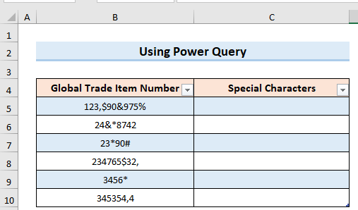
Step 1: Locating Your Data Table
Your first task involves finding the data table containing the Global Trade Item Number in Column B and the Special Characters in Column C.
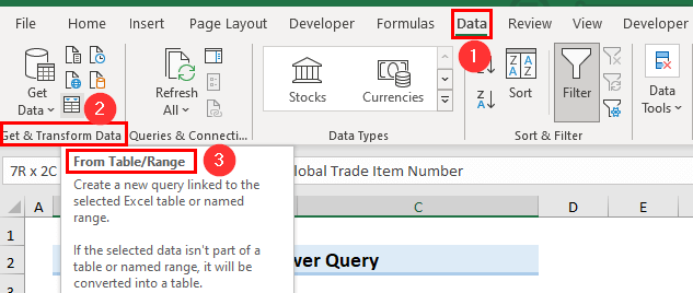
Step 2: Initiating Data Transformation
Head over to the Data tab and select the Get & Transform Data option. From the dropdown menu, choose From Table/Range to initiate the data transformation process.
Step 3: Creating a Custom Column
Within the newly opened Table2 window, proceed to the Add Column tab and select the Custom Column option.

Step 4: Implementing the Custom Column Formula
Inside the Custom Column window, insert the following formula into the designated field:
=Text.Remove([Global Trade Item Number],{“A”..”z”,”0″..”9″})

After inputting the formula, click OK to witness the results.

Step 5: Finalizing the Process
With your newly created column in place, conclude the process by clicking the Close & Load option found in the Home tab.

Step 6: Reveling in the Results
Marvel at the results of your efforts as the special characters are meticulously identified and extracted. Your data presentation has now reached an unparalleled level of excellence.

Method 2: Employing VBA Code for Detecting Special Characters
For those who prefer to delve into coding territory, VBA offers an ingenious solution. Follow these steps to wield VBA code for special character detection:
Step 1: Accessing the VBA Window
Begin by opening the VBA window, which can be achieved by pressing Alt+F11.
Step 2: Incorporating the VBA Code
Navigate to the Insert tab within the VBA window and select the Module option.

Within the newly created module, insert the following VBA code:
Function FindSpecialCharacters(TextValue As String) As Boolean
Dim Starting_Character As Long
Dim Acceptable_Character As String
For Starting_Character = 1 To Len(TextValue)
Acceptable_Character = Mid(TextValue, Starting_Character, 1)
Select Case Acceptable_Character
Case “0” To “9”, “A” To “Z”, “a” To “z”, ” ”
FindSpecialCharacters = False
Case Else
FindSpecialCharacters = True
Exit For
End Select
Next
End Function

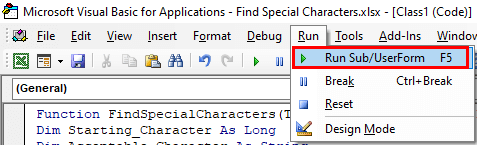
After inserting the code, put it to the test by clicking the Run option (F5) to check for any errors in your VBA code.
Step 4: Saving Your Creation
With your code verified, save it by pressing Ctrl+S. Your masterpiece is now safely stored for future use.
Step 5: Implementing the Code
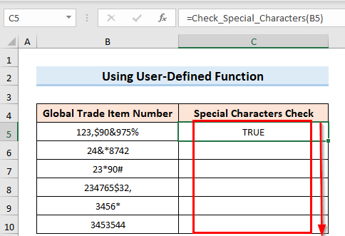
Return to your main worksheet and proceed to the C5 cell. Input the following formula to apply your newly minted code:
=FindSpecialCharacters(B5)
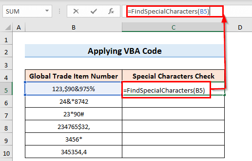
Upon entering the formula, the outcome will be revealed. A TRUE value will signify the presence of special characters within the cell.
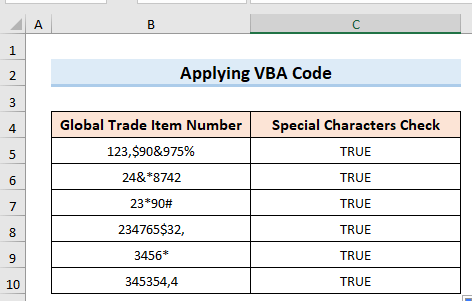
Step 6: Extending the Functionality
Extend this function across your sheet using the Fill Handle to populate the remaining cells in the same column.
Step 7: Embracing the Outcome
The results are in, and your Excel sheet now effortlessly identifies the presence of special characters, ensuring the accuracy and integrity of your data.
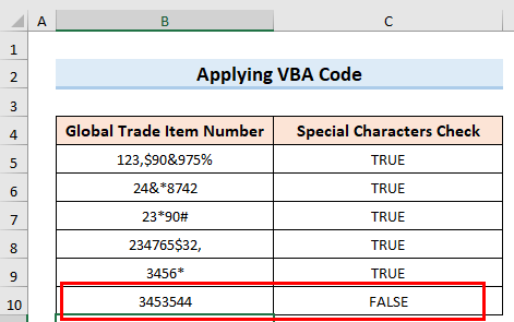
If alterations are made to data containing no special characters, the result displayed in the box will be FALSE.
Conclusion:
By unveiling these two dynamic methods, your journey to identifying special characters in Excel takes a quantum leap. Whether you opt for the intuitive Power Query route or the code-driven VBA approach, your data presentations are primed for excellence. No more ambiguities or overlooked nuances – just pure, unadulterated data brilliance.