Excel, with its powerful data management and calculation capabilities, is a popular choice for professionals and individuals alike. One of the key aspects of data presentation is how you handle zero values.
Sometimes, you might want to hide these zero values to enhance the visual appeal of your worksheets and create a more polished and professional-looking data set. In this tutorial, we will delve into the various methods to hide zero values in Excel, offering you greater flexibility in presenting your data.
Method 1: Hiding Zero Values Using Excel Options
Excel provides users with a built-in feature that automatically hides all zero values within an entire worksheet. This method is particularly useful when you wish to conceal all instances of zero values in your data set. To utilize this feature, follow these steps:
- Open the workbook containing the worksheet where you want to hide zero values.
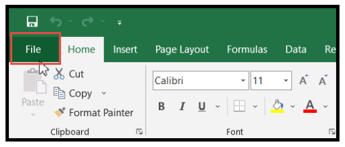
- Click on the File tab in the top-left corner of the Excel window.
- From the dropdown menu, select Options.

- In the Excel Options dialog box, choose the Advanced category from the left pane.
- Scroll down to find the “Display options for this worksheet” section.
- Locate the checkbox that says “Show a zero in cells that have zero value” and uncheck it.
- Click OK to apply the changes.

By following these straightforward steps, all the zero values in the selected worksheet will be hidden, and the corresponding cells will appear blank.

This method ensures that your data presentation remains clean and uncluttered, making it easier for viewers to focus on essential information.
Method 2: Hiding Zero Values in Selected Cells Using Format Cells
If you prefer more granular control over which zero values to hide, Excel’s custom formatting feature is the ideal solution. This method allows you to specify how Excel displays different types of numbers, including zero values, within the selected cells or data range. To apply custom formatting to hide zero values, follow these steps:
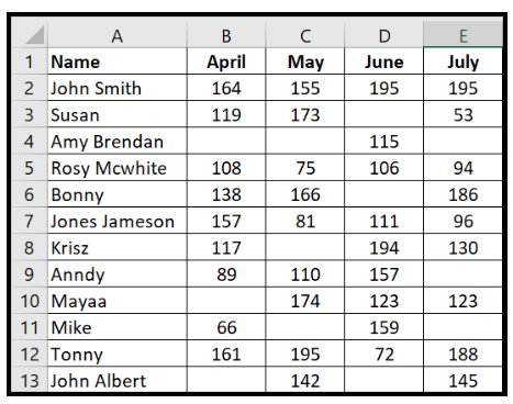
- Select the cells or data range where you want to hide the zero values.
- Right-click on the selection to open the context menu.
- From the menu, choose Format Cells to open the Format Cells dialog box.

- In the Format Cells dialog box, navigate to the Number tab.
- Within the Category list, select Custom.
- In the Type field, enter the custom format: 0;-0;;@.

- Click OK to apply the custom format.

The custom format 0;-0;;@ consists of four parts:
- The first 0 instructs Excel to display positive numbers as they are, without any modification.
- The second -0 directs Excel to display negative numbers as they are, retaining their original format.
- The third 0 is missing in the format, which effectively hides zero values, making the cells look blank.
- The fourth @ is used to display text as is, without any changes.
By utilizing this custom format, all the zero values within the selected range will be hidden, providing a clear and refined appearance to your data.
Method 3: Hiding Zero Values in Selected Cells Using Conditional Formatting
Excel’s conditional formatting feature empowers you to dynamically change the appearance of cells based on specific conditions. This method is particularly useful when you want to visually identify cells containing zero values without altering the actual data. To apply conditional formatting to hide zero values, follow these steps:
- Select the cells or data range where you want to hide the zero values.
- Navigate to the Home tab on the Excel ribbon.
- Click on the Conditional Formatting icon to access the Conditional Formatting menu.
- Choose Highlight Cells Rules from the menu and then select Equal To.

- In the left-side field of the Equal To dialog box, enter (0) to specify that you want to format cells that are equal to zero.
- Click on the drop-down on the right side of the dialog box and choose Custom Format.

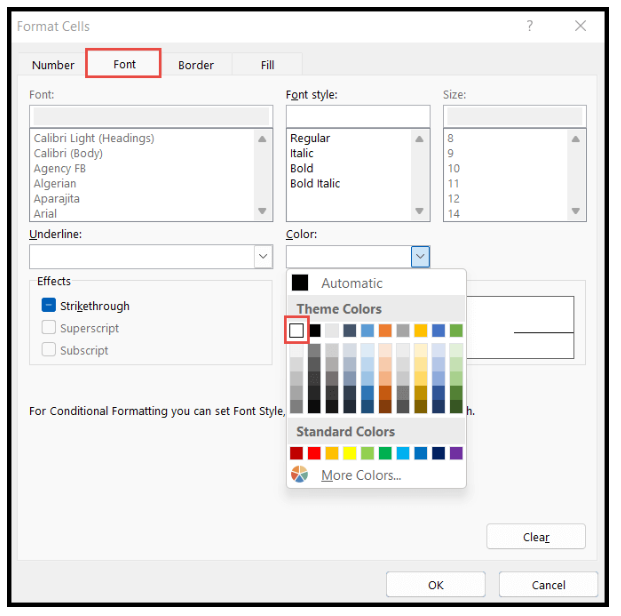
- In the Format Cells dialog box, navigate to the Font tab and choose the white color for the font.
- Click OK to apply the conditional formatting.
By implementing this conditional formatting rule, the font color of cells containing zero values will become white, effectively making the cells look empty or blank while preserving the underlying data.
Please note that hiding zero values using conditional formatting is purely a visual effect and does not affect the actual data. The zero values remain in the cells, ensuring data accuracy and integrity.
Conclusion
In conclusion, Excel offers a range of options to hide zero values, providing you with the flexibility to present your data in a more visually appealing manner.
Whether you want to hide zero values throughout an entire worksheet or selectively in specific cells, Excel’s diverse features have you covered. By employing these methods, you can enhance the aesthetics of your data and create impressive reports and presentations with ease. So go ahead, experiment with these techniques, and take your Excel skills to the next level!