Whether you’re a seasoned Excel user or just starting to explore the vast possibilities of this powerful spreadsheet software, understanding how to visually highlight negative numbers can greatly enhance the clarity and impact of your data analysis.
Excel provides various formatting options to manipulate cells, and one of the most effective ways to draw attention to negative values is by changing their color to red. By following the step-by-step instructions in this blog post, you’ll learn not only how to highlight negative numbers in Excel but also how to customize the formatting to suit your specific needs.
From simple conditional formatting rules to advanced formulas and techniques, we’ll equip you with the knowledge and skills necessary to transform your data into visually appealing and easily interpretable worksheets. So let’s dive right in and discover the secrets to making negative numbers red in Excel!
Different Methods to Make Negative Numbers Red in Excel
Method 1: Conditional Formatting
Conditional formatting in Excel enables you to apply formatting rules based on cell values. Follow these steps to highlight negative numbers in red:
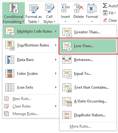
- Step 1: Access Conditional Formatting: Navigate to the “Home” tab, locate the “Conditional Formatting” option in the ribbon, and select “Highlight Cell Rules.”
- Step 2: Choose “Less Than”: From the provided options, select “Less Than” to create a rule that identifies cells with values lower than a specified threshold.
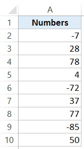
- Step 3: Select the Cells: Now select the cells that contain the negative numbers which you want to make red
- Step 4: Specify the Threshold: In the “Less Than” dialog box, enter “0” as the threshold value. If desired, you can customize the formatting using the “Custom Format” option.
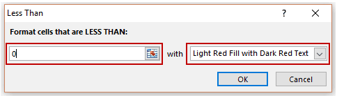
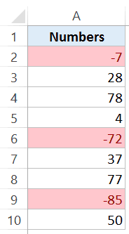
Step 5: Apply the Formatting: Click “OK” to apply the conditional formatting. All cells containing values below 0 will be highlighted in a distinctive red color, ensuring easy identification.
Utilizing conditional formatting not only enhances the appearance of your data but also proves beneficial when generating printed reports. Even in black and white printouts, the highlighted cells stand out, facilitating clear data interpretation.
Note: Keep in mind that conditional formatting is a dynamic feature that recalculates whenever changes are made to the workbook. While its impact is minimal on smaller datasets, it may slightly affect performance when applied to larger datasets.
Method 2: Inbuilt Excel Number Formatting
Excel provides built-in number formatting options that simplify the process of highlighting negative numbers in red. Follow these steps to utilize this feature:
- Step 1: Select the Relevant Cells: Choose the cells where you want to highlight negative numbers in red.
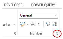
- Step 2: Access the Format Cell Dialog Box: Go to the “Home” tab and locate the “Number Format” group. Click on the dialog launcher icon (the small tilted arrow icon at the bottom right of the group) or use the keyboard shortcut Control + 1.
- Step 3: Choose the Number Format: Within the “Format Cells” dialog box, switch to the “Number” tab. From the “Category” list, select “Number.” On the right side, choose the option that displays negative numbers in red text.
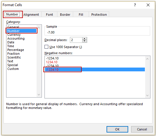
- Step 4: Apply the Formatting: Click “OK” to apply the number formatting. The selected cells will now display negative numbers with two decimal places and appear in red, making them visually distinct.
It’s important to understand that these formatting techniques do not alter the actual values within the cells. They solely affect the visual representation of the numbers while preserving their original values.
Conclusion
In conclusion, knowing how to make negative numbers red in Excel can significantly enhance the visual presentation and interpretation of your data. By following the steps outlined in this guide, you have learned different methods to highlight negative values and customize their formatting according to your preferences.
Whether you opt for simple conditional formatting rules or utilize more advanced formulas, you now have the tools at your disposal to create visually appealing and informative worksheets. Remember that effective data analysis involves not only accurate calculations but also clear communication, and highlighting negative numbers in red can help you achieve just that.
So go ahead and apply these techniques to your Excel projects, and watch as your data comes to life with clarity and impact. With practice and experimentation, you’ll become proficient in leveraging Excel’s formatting capabilities to effectively convey your insights to others. Happy Excel-ing!