When it comes to working with numbers in Excel, the possibilities seem endless. From basic calculations to complex formulas, Excel provides users with a wide range of tools to handle numerical data efficiently.
However, dealing with negative numbers can sometimes pose a challenge, especially when you need to add them up. Do you want to know how to sum negative numbers in Excel? Whether you’re new to Excel or an experienced user looking to enhance your skills, this blog post will guide you step by step on how to add up negative numbers in Excel.
We’ll explore different techniques, formulas, and tips that will empower you to confidently perform calculations involving negative numbers and achieve accurate results. So, let’s dive in and discover the simple yet effective methods that Excel offers for adding negative numbers in Excel.
Method 1: Use of SUMIF Function to Add Negative Numbers in Excel
The SUMIF function in Excel allows you to add specific numbers based on given criteria. By utilizing this function, you can add negative numbers effortlessly. Follow the steps below to implement this method:
Steps:
- Select a cell where you want the result to be displayed. Let’s choose cell C11 as an example.
- In the selected cell (C11), enter the following formula:
=SUMIF(C5:C10, “<0”, C5:C10)

- Remember to enclose the criteria in double quotation marks when not referring to a specific cell value.
- Finally, press ENTER to view the added negative number in cell C11.

Method 2: Applying AutoSum Feature for Adding Negative Numbers
Excel provides a convenient feature called AutoSum, which includes various functions for automated calculations. By utilizing the SUM function within AutoSum, you can effortlessly add negative numbers. Follow the steps below to implement this method:
Steps:
- Select the cell (C11) where you want the sum to appear.
- Navigate to the Home tab and click on the Editing command.
- From the AutoSum drop-down menu, choose the SUM function.

- Excel will automatically select the data range to be summed up based on your selection.

- Press ENTER, and you will see the added negative number in cell C11.

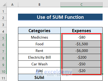
Method 3: Employing Format Cells Command and SUM Function
Formatting cells can enhance the visual representation of data in Excel. By using the Format Cells command and the SUM function, you can format negative numbers and add them efficiently. Follow the steps below to implement this method and you’ll get to know how to sum all negative numbers in Excel:
Steps:
- Select the data range you want to format, such as C5:C10.
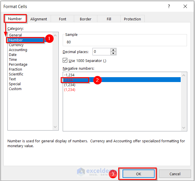
- To open the Format Cells dialog box directly, press the CTRL+1 keys.
- In the Format Cells dialog box, ensure that you are on the Number tab.
- Select the Currency option if you want to keep the dollar sign for monetary values.
- Under the “Negative numbers” section, choose your preferred style. For example, select the 2nd style.
- Press OK to apply the changes.

- If you want to keep the data as numbers only, choose the Number format in Step 4 and select the desired style for negative numbers.
- Now, select a different cell (C11) where you want the result to be displayed.
- In the selected cell (C11), enter the following formula:
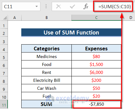
=SUM(C5:C10)
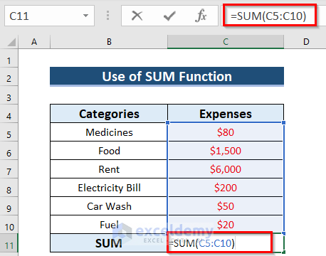
- Press ENTER, and you will see the added negative number in cell C11.

Method 4: Generic Formula to Add Negative Numbers in Excel
If you prefer a manual approach, you can use a generic formula to add negative numbers in Excel. This method allows you to directly sum up the cell values using the plus (+) sign. Follow the steps below to implement this method and ultimately the formula to sum all negative numbers in Excel will give you the desired results:
Steps:
- Select a cell (C11) where you want the result to be displayed.
- In the selected cell (C11), enter the following formula:
=C5 + C6 + C7 + C8 + C9 + C10
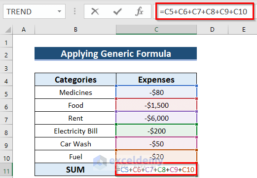
- Press ENTER, and you will see the added negative number in cell C11.

The Bottom Line
By following the techniques and tips outlined in this blog post, you can confidently tackle calculations involving negative numbers and obtain accurate results.
Whether you prefer using basic arithmetic operations, the SUM function, or specialized formulas like SUMIF and SUMIFS, Excel provides a versatile set of tools to handle negative numbers efficiently.
Remember to keep track of the signs of your numbers, use parentheses when necessary, and leverage the power of Excel’s functions and formulas to simplify your calculations. This is how to sum negative numbers in Excel effortlessly.
With practice and familiarity, you’ll become proficient in working with negative numbers in Excel, saving time and effort in your data analysis tasks. So, start applying these methods today and unlock the full potential of Excel’s number-crunching capabilities.