How to fix a circular reference in Excel is a query that comes up in almost every user’s mind. Before going to answer it let’s understand what this error is in reality.
Excel has many basic as well as advanced tools to be used for increased productivity and better performance. Using formulas, you can make more and more advanced calculations smoothly. On the other hand, one thing you must keep in your mind is when the complexity level goes up, the chances of facing any problem also rise.
Having a huge dataset brings more complexity to it. However, Excel never makes your tasks trickier because it has multiple features to ease the calculations. When entering some formula in an Excel sheet and it is not working, there could be something wrong with that formula. By default, you will see a message on the screen about a circular reference.
A circular reference is something that thousands of users face every day. It happens just because an Excel formula is being forced to calculate its own cell. If by mistake or intentionally you do it, you will see Excel notifies you with a message on the screen that says:
“Careful, we found one or more circular references in your workbook which might cause your formula to calculate incorrectly.”
Define a Circular Reference
A circular reference appears when a formula tries to calculate itself. In more simple words, when a formula is referred to the same cell in which it is placed and referring loop pressurizes the formula to act without completion.
How to Fix a Circular Reference in Excel?
Fixing an error never ends up in just a single step; you always have to go through several clicks to completely vanish the problem. Similarly, fixing a circular reference will need you to follow multiple steps, so that you can finish the task properly. You might have to trace them back to start fixing the formula. Or else you can remove them one by one.
We have two methods for tracing to remove circular references by tracing relationships between formulas and cells.
Follow the steps given below:
-
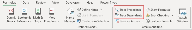
Open the Formulas tab in Excel
You will see two options there named Trace Precedents and Trace Dependents.
Following these steps can let you fix circular references by connecting the references through a line. This line usually appears in between the cells responding to the circular references.
Let’s understand how these two tracing options work:
1. Trace Precedents
This feature tracks back cells that are dependent on the current cell. The current formula is dependent on these cells for the data and using this option lets you draw lines that clearly show the affected active cells.
Below you can see an example, in which the cells are affecting B5, B2, B3, and B4. When you click on the Trace Precedents, you will see a line indicating B2, B3, and B5.

Shortcut for Trace Precedents: ALT + TUT
2.Trace Dependents
Using this feature lets you track the dependent cells that are active and the cells that are dependent on the current cell for the data. You will also see lines to the cells that are dependent on the active cells.
Below in the given example, you will see the affected cell by B5 and B4. B5 is dependent on its value, that’s why when the trace dependents feature is used, a line from B5 to B4 is drawn, which shows that B4 is dependent on B5.
Shortcut for Trace Dependents: ALT+TUD
Now, the procedure for solving the query of how to fix a circular reference in Excel is completed. You must be having a clear idea about how you can fix this issue without involving in a mess. By now, you have a good approach toward how circular references work and how you can fix them.